core

The core module.

Note

The following developments comply with the YAGNI principle without sacrificing any axis of generalization.

Warning

Variables’ notations only serve a distinctive purpose and will be revised.

Todo

Add MyPy-friendly type annotations.

class iamax.core.DSpace(file_path: str = '', sheets_names: dict = None, year: str|int = BASE_YEAR, **kwargs: 'str')

Class that aggregates a bunch of attributes and methods related to the dimensionality-agnostic assimilation of the dataspace.

Parameters

• file_path (str) – Full path of the excel file to read, be it absolute or relative. Set to '' by default.

• year (int or str) – Location of the instance onto the (discrete) temporal line of years. Set to BASE_YEAR by default.

• sheets_names (dict) – Correspondences between worksheets’ internal names and their external counterpart. Set to None by default.

Note

As just outlined, argument sheets_names consists in a python dictionary whose i) keys relate to data’ internal names and ii) values to the arbitrary ones that users have chosen. A non-exhaustive (tabulated) list follows.

sheets_names’s key	Meaning
consumer_prices	Consumption prices
excises_totals	Excises values
excises_exorates	Excises exoneration rates
income_private_circuit	Income private | circuit
input_values	Input costs
input_volumes	Input volumes
markets_rents	Markets driven rents
contrib_taxes	Contributive taxes
output_volumes	Output volumes
output_values	Output values
producer_gross_prices	Average gross producer price
producer_net_prices	Average net producer price
sales_taxes_totals	Sales taxes | totals
sales_taxes_exorates	Sales taxes exoneration rates
specific_margins	Specific margins
unemployment_rates	Unemployed capacities rates
mappings_trees	Per entity morphism

If you want to provide your DSpace instance with information regarding how each datum evolve over time, you can either

1. Directly long-format your tables or

2. Provide your tables as wide and then create another sheet displaying (0-centered) rates of growth.

If you decide to go the second way, the instantiation argument is that of the sheet name of interest suffixed with '_grates'. See the example below.

In the exact same fashion, you can also endow your data with (an other type of) 0-centered components, suffixing with '_drates' instead, standing ‘driving’ rates.

Important

The above table is not exhaustive. To get a full list of the sheets names that can be used, you can call display_legal_sheets_names(), refer to it.

Example

>>> system = DSpace(  
...     file_path='examples/.ut(KLEM-BRICS-202006)-fr.xlsx',
...     sheets_names={
...         'input_volumes'        : "volumes intrant",
...         'input_values'         : "valeurs des intrants",
...         'markets_rents'        : "rentes économiques",
...         'producer_gross_prices': "prix bruts de production",
...         'consumer_prices'      : "prix à la consommation",
...         'output_volumes'       : "volumes extrant",
...         'contrib_taxes'        : "taxes contributives",
...         'excises_totals'       : "accises",
...         'excises_exorates'     : "taux d'éxonération d'accises",
...         'sales_taxes_totals'   : "TVA",
...         'sales_taxes_exorates' : "taux d'éxonération de TVA",
...         'specific_margins'     : "marges spécifiques",
...         'unemployment_rates'   : "surcapacités relatives",
...         'mappings'             : "entities",
...     }
... )

Echoing the advices related to growth rates, the following shows the way to go.

>>> system = DSpace(  
...     file_path='examples/.ut(KLEM-BRICS-202006)-fr.xlsx',
...     sheets_names={
...         ...
...         'specific_margins': "marges spécifiques",  # Wide
...         'specific_margins_grates': "dynamique des marges",  # Long
...         ...
...     }
... )

classmethod display_legal_sheets_names(cls)

Helper defined to display the legal arguments names to be used when getting a DSpace (or MSystem) instance.

Example

>>> DSpace.display_legal_sheets_names()  
added_values
added_values_drates
 ...
utilization_rates_grates
utilization_rates_lagged
utilization_rates_shoptr

property uid(self)

Dataquest unique identifier.

Note

This attribute is session-stable and cross-platform.

Example

>>> DSpace().uid
'mvYPyV7vwEpp'

property _keyed_core_sheets_names(self)

Keyed sheets’ names whose content consist in numerical data.

Note

This attribute is not intended for public use.

Example

>>> s = DSpace(
...     'examples/ut(KLEM-BRICS-202006)@sol.xlsx', {
...         'input_values': 'i-vals',
...         'mappings': 'entities',
...     }
... )
>>> s._keyed_core_sheets_names
{'_ivals': 'i-vals'}

property _keyed_epi_sheets_names(self)

Keyed sheets’ names whose content consist in epi-data.

Note

This attribute is not intended for public use.

Example

>>> s = DSpace(
...     'examples/ut(KLEM-BRICS-202006)@sol.xlsx', {
...         'input_values': 'i-vals',
...         'mappings': 'entities',
...     }
... )
>>> s._keyed_epi_sheets_names
{'mppngs': 'entities'}

property _keyed_sheets_names(self)

Merging of _keyed_core_sheets_names and _keyed_epi_sheets_names attributes.

Note

This attribute is not intended for public use.

Example

>>> s = DSpace(
...     'examples/ut(KLEM-BRICS-202006)@sol.xlsx', {
...         'input_values': 'i-vals',
...         'mappings': 'entities',
...     }
... )
>>> s._keyed_sheets_names
{'_ivals': 'i-vals', 'mppngs': 'entities'}

property _named_sheets_keys(self)

_keyed_sheets_names’s reciprocal.

Note

This attribute is not intended for public use.

Example

>>> s = DSpace(
...     'examples/ut(KLEM-BRICS-202006)@sol.xlsx', {
...         'input_values': 'i-vals',
...         'mappings': 'entities',
...     }
... )
>>> s._named_sheets_keys
{'i-vals': '_ivals', 'entities': 'mppngs'}

_sheet_ids_getter(self, sheet_name_or_key: str, on_error: str = 'raise')

Get pairs of (public and private) names associated to a sheet’s (public or private) name.

Parameters

• sheet_name_or_key (str) – Public or internal/private name of the worksheet to be identified.

• on_error (str) – Behavior to be adopted by the method in case of error. Options are 'raise', 'ignore' and 'warn'. Set to 'raise' by default.

Note

This method is not intended for public use.

Example

>>> s = DSpace(
...     'examples/ut(KLEM-BRICS-202006)@sol.xlsx', {
...         'input_values': 'i-vals',
...         'mappings': 'entities',
...     }
... )
>>> s._sheet_ids_getter(
...     sheet_name_or_key='_ivals'
... )
('i-vals', '_ivals')
>>> s._sheet_ids_getter(
...     sheet_name_or_key='i-vals'
... )
('i-vals', '_ivals')
>>> s._sheet_ids_getter(
...     sheet_name_or_key='input sales', on_error='ignore'
... )
(None, None)

property _grates_keys(self)

Growth rates variables’ private names.

Note

This attribute is not intended to be used publicly.

property _grates_saturations_keys(self)

Growth rates saturations variables’ private names.

Note

This attribute is not intended to be used publicly.

property _drates_keys(self)

Driving rates variables’ private names.

Note

This attribute is not intended to be used publicly.

property _lagged_keys(self)

Lagged variables’ private names.

Note

This attribute is not intended to be used publicly.

property file_as_xml_obj(self)

Instance of Archiver that concentrates all metadata that can be gathered from the instantiation input file.

Example

>>> md = DSpace(
...     'examples/ut(KLEM-BRICS-202006)@sol.xlsx',
...     sheets_names={'input_values': 'i-vals'}
... ).file_as_xml_obj['i-vals']
>>> md.keys()
dict_keys(['styles', 'comments', 'hyperlinks'])

See also

iloc_styles(), iloc_hyperlinks() and iloc_comments().

property file_as_pd_obj(self)

Caching wrapper of xl_file_getter() configured with a 'pandas' engine.

Example

>>> DSpace(
...     'examples/ut(KLEM-BRICS-202006)@sol.xlsx',
... ).file_as_pd_obj  
{
   ...
  "language": "en-US",
   ...
}

property file_as_op_obj(self)

Caching wrapper of xl_file_getter() configured with a 'openpyxl' engine.

Example

>>> DSpace(
...     'examples/ut(KLEM-BRICS-202006)@sol.xlsx',
... ).file_as_op_obj  
{
   ...
  "language": "en-US",
   ...
}

_close(self)

Close all file’s working accesses.

Example

>>> ds = DSpace(
...     'examples/ut(KLEM-BRICS-202006)@sol.xlsx'
... )
>>> ds._close()

table_reader(self, sheet_name: str, **kwargs: type)

Augmented wrapper of xl_ndtables_pd_reader().

Parameters

• sheet_name (str) – Name of the sheet that contains data.

• **kwargs (type) – xl_ndtables_pd_reader() remaining arguments.

Example

>>> s = DSpace(
...     'examples/ut(KLEM-BRICS-202006)@sol.xlsx',
... )
>>> df = s.table_reader(
...     sheet_name='sp-mgs', frame_addrs=True, dropna=True
... )
>>> df
               n
               z                     d                    x
           o_kle      e_kle          c    g    i          e
n a e  826457.27 -731385.37 -202822.61  0.0  0.0  107750.71
>>> df.attrs['addresses']
          n
          z         d           x
      o_kle e_kle   c   g   i   e
n a e    D4    E4  F4  G4  H4  I4

property _localization(self)

Position of the DSpace instance in hand within _localizations.

Example

>>> DSpace()._localization
MultiIndex([(2010,)],
           names=['year'])
>>> DSpace(year=1010)._localization
MultiIndex([(1010,)],
           names=['year'])

property _localization_delta(self)

Position of the DSpace instance in hand within _localizations_deltas.

Example

>>> DSpace()._localization_delta
MultiIndex([(0.0,)],
           names=['year'])
>>> DSpace(year=1010)._localization_delta
MultiIndex([(0.0,)],
           names=['year'])

property _ilocalization(self)

Integer-based version of _localization,

See also

_χ and t.

Example

>>> DSpace()._ilocalization
0
>>> DSpace(year=1010)._ilocalization
0

>>> s = DSpace(
...     'examples/ut(KLEM-BRICS-202006)@sol.xlsx', year=2020,
...     sheets_names={'input_volumes': 'i-vols'}
... )
>>> s._localizations
MultiIndex([(2010,),
            (2015,),
            (2020,),
            (2025,),
            (2030,),
            (2035,),
            (2040,),
            (2045,),
            (2050,)],
           names=['year'])
>>> s._localization
MultiIndex([(2020,)],
           names=['year'])
>>> s._ilocalization
2

>>> s.year = 2045
>>> s._localization
MultiIndex([(2045,)],
           names=['year'])
>>> s._ilocalization
7

property _χ(self)

_ilocalization’s alias.

property _к(self)

Discretized _ilocalization’s version that qualifies the current modeling phase, between Calibration and Recursion.

Example

>>> DSpace()._к
'C'

property t(self)

Yet another _ilocalization’s alias, vanishing the generality by restricting the evolution domain of data to that of time.

See also

_χ.

property year(self)

Getter/setter specifying the position of the instance in hand onto one of the _localizations’s dimension, i.e. that related to year.

Example

>>> DSpace().year
2010

Why 2010 ? Remember BASE_YEAR.

>>> s = DSpace(year=1990)
>>> s.year
1990
>>> s.year = 2100
>>> s._year
2100

property _dlocalization(self)

Difference between two consecutive _localization.

See also

_dγ, delta_year and dyear.

Example

>>> DSpace()._dlocalization
Array(0., dtype=float64)
>>> DSpace(year=1010)._dlocalization
Array(0., dtype=float64)

>>> s = DSpace(
...     'examples/ut(KLEM-BRICS-202006)@sol.xlsx', year=2020,
...     sheets_names={'input_volumes': 'i-vols'}
... )
>>> s._ilocalization
2
>>> s._localization
MultiIndex([(2020,)],
           names=['year'])
>>> s._dlocalization
Array(5., dtype=float64)

property _dγ(self)

_dlocalization’s alias.

property delta_year(self)

Yet another _dlocalization’s alias, vanishing the generality by expliciting the evolution domain of data to that of time.

See also

_dγ and _dlocalization.

property dyear(self)

Yet another _dlocalization’s alias.

See also

delta_year.

property _raw_nodes(self)

Dictionary of nodes read from the tab related to entities’ technology/preference/behavior/dynamic.

Example

>>> DSpace()._raw_nodes
[]

>>> DSpace(
...     'examples/ut(KLEM-BRICS-202006)@sol.xlsx',
...     dict(mappings='entities'),
... )._raw_nodes  
[((('n', 'd', 'k'),), Node...)]

property _blueprint(self, _usym: str = UNIV_SYM)

Largest possible data space – built over provided sheets – and rendered as _localizations-indexed square matrices.

Parameters

_usym (str) – Unaccessible argument defined at the class level. Set to UNIV_SYM.

Example

>>> DSpace()._blueprint
Empty DataFrame
Columns: []
Index: [(2010,)]

>>> DSpace(
...     'examples/ut(KLEM-BRICS-202006)@sol.xlsx',
...     sheets_names={'sales_taxes_totals': 's-txs-tot'}
... )._blueprint
              *    n
              *    a
              *    e    o
year
2010 * * *  0.0  0.0  0.0
     n a e  0.0  0.0  0.0
         o  0.0  0.0  0.0

>>> DSpace(
...     'examples/ut(KLEM-BRICS-202006)@sol.xlsx',
...     sheets_names={'input_volumes': 'i-vols'}
... )._blueprint.iloc[:10, :5]
              *    n
              *    a    d
              *    e    c    g    i
year
2010 * * *  0.0  0.0  0.0  0.0  0.0
     n a e  0.0  0.0  0.0  0.0  0.0
       d c  0.0  0.0  0.0  0.0  0.0
         g  0.0  0.0  0.0  0.0  0.0
         i  0.0  0.0  0.0  0.0  0.0
       m e  0.0  0.0  0.0  0.0  0.0
       x e  0.0  0.0  0.0  0.0  0.0
2015 * * *  0.0  0.0  0.0  0.0  0.0
     n a e  0.0  0.0  0.0  0.0  0.0
       d c  0.0  0.0  0.0  0.0  0.0

property _loc_blueprint(self)

Localized version of _blueprint.

Example

>>> DSpace()._loc_blueprint
Empty DataFrame
Columns: []
Index: []

>>> DSpace(
...     'examples/ut(KLEM-BRICS-202006)@sol.xlsx',
...     sheets_names={'sales_taxes_totals': 's-txs-tot'}
... )._loc_blueprint
         *    n
         *    a
         *    e    o
* * *  0.0  0.0  0.0
n a e  0.0  0.0  0.0
    o  0.0  0.0  0.0

property _identifiers(self)

Label space the good-and-service’s index set \(\mcI\) (cf. Eq.1) derives from.

Example

The identifiers space has to be representative of something, which is why we instantiate DSpace below with at least one sheet, whatever it is as long as it relates to rectangular data.

>>> DSpace(
...     'examples/ut(KLEM-BRICS-202006)@sol.xlsx', sheets_names={
...         'sales_taxes_exorates': '¬%(s-txs)'
...     }
... )._identifiers
MultiIndex([('*', '*', '*'),
            ('n', 'a', 'e'),
            ('n', 'a', 'o'),
            ('n', 'x', 'e'),
            ('n', 'x', 'o')],
           )

property _identifiers_space(self)

_identifiers’s alias.

property _identifiers_exp(self)

Explicitly active entities’ identifiers.

Example

>>> DSpace(
...     'examples/ut(KLEM-BRICS-202006)@sol.xlsx', sheets_names={
...         'sales_taxes_exorates': '¬%(s-txs)'
...     }
... )._identifiers_exp
MultiIndex([('n', 'a', 'e'),
            ('n', 'a', 'o'),
            ('n', 'x', 'e'),
            ('n', 'x', 'o')],
           )

property _identifiers_imp(self)

Implicitly active entities’ identifiers.

Example

>>> DSpace(
...     'examples/ut(KLEM-BRICS-202006)@sol.xlsx', sheets_names={
...         'mappings': 'entities',
...         'input_values': 'i-vals'
...     }
... )._identifiers_imp
MultiIndex([('n', 'b',   'b'),
            ('n', 'd',  'cg'),
            ('n', 'd', 'cgi'),
            ('n', 'd',  'ib'),
            ('n', 'd',   'l'),
            ('n', 'm',   '*'),
            ('n', 'n',   'n'),
            ('n', 'x',   '*')],
           )

property _iidentifiers(self)

_identifiers’s index set, denoted as

(1)\[\mcI = \{ n \mid n \in \mathbb{N} \}\]

Note

\(\mcI\)’s python archetype is stricto sensu not a set, but a tuple.

Example

>>> DSpace(
...     'examples/ut(KLEM-BRICS-202006)@sol.xlsx', sheets_names={
...         'sales_taxes_exorates': '¬%(s-txs)'
...     }
... )._iidentifiers
(0, 1, 2, 3, 4)

property _identifiers_card(self)

Cardinality of the label space, \(|\mcI|\).

Example

>>> DSpace(
...     'examples/ut(KLEM-BRICS-202006)@sol.xlsx', sheets_names={
...         'sales_taxes_exorates': '¬%(s-txs)'
...     }
... )._identifiers_card
5

property _identifiers_ndim(self)

Dimensionality of the label space.

Example

>>> DSpace(
...     'examples/ut(KLEM-BRICS-202006)@sol.xlsx', sheets_names={
...         'sales_taxes_exorates': '¬%(s-txs)'
...     }
... )._identifiers_ndim
3

property _identifiers_right_levels_range(self)

Identifying right levels’ integer positions.

Example

>>> DSpace(
...     'examples/ut(KLEM-BRICS-202006)@sol.xlsx', sheets_names={
...         'sales_taxes_exorates': '¬%(s-txs)'
...     }
... )._identifiers_right_levels_range
[-3, -2, -1]

property _identifiers_left_levels_range(self)

Identifying left levels’ integer positions.

Example

>>> DSpace(
...     'examples/ut(KLEM-BRICS-202006)@sol.xlsx', sheets_names={
...         'sales_taxes_exorates': '¬%(s-txs)'
...     }
... )._identifiers_left_levels_range
[1, 2, 3]

property _identifiers_left_loc_levels_range(self)

Identifying left levels’ localized integer positions.

Example

>>> DSpace(
...     'examples/ut(KLEM-BRICS-202006)@sol.xlsx', sheets_names={
...         'sales_taxes_exorates': '¬%(s-txs)'
...     }
... )._identifiers_left_loc_levels_range
[0, 1, 2]

property _identifiers_hyperplanes(self)

Label space’s hyperplanes.

See also

Why is a Hyperplane called a “Hyper”plane?

Example

The identifiers space has to be representative of something, which is why we instantiate DSpace below with at least one sheet, whatever it is as long as it relates to rectangular data.

>>> s = DSpace(
...     'examples/ut(KLEM-BRICS-202006)@sol.xlsx', sheets_names={
...         'sales_taxes_exorates': '¬%(s-txs)'
...     }
... )
>>> s._identifiers_hyperplanes[0]
MultiIndex([('*',),
            ('n',),
            ('n',),
            ('n',),
            ('n',)],
           )
>>> s._identifiers_hyperplanes[1]
MultiIndex([('*', '*'),
            ('n', 'a'),
            ('n', 'a'),
            ('n', 'x'),
            ('n', 'x')],
           )

Cf. _identifiers if you haven’t already.

property _univ_identifiers(self, _usym: str = UNIV_SYM)

Archetype of the (CSS inspired) universal index, ordered by level from 0 to _identifiers_ndim.

Parameters

_usym (str) – Unaccessible argument defined at the class level. Set to UNIV_SYM.

Example

>>> DSpace()._univ_identifiers
[Index([], dtype='object')]

>>> s = DSpace(
...     'examples/ut(KLEM-BRICS-202006)@sol.xlsx',
...     sheets_names={'sales_taxes_totals': 's-txs-tot'}
... )
>>> s._univ_identifiers[0]
MultiIndex([('*',)],
           )
>>> s._univ_identifiers[1]
MultiIndex([('*', '*')],
           )
>>> s._univ_identifiers[-1]
MultiIndex([('*', '*', '*')],
           )

property _loc_univ_identifiers(self, _usym: str = UNIV_SYM)

Localized version of _univ_identifiers.

Parameters

_usym (str) – Unaccessible argument defined at the class level. Set to UNIV_SYM.

Example

>>> DSpace()._loc_univ_identifiers[0]
MultiIndex([(2010,)],
           names=['year'])

>>> s = DSpace(
...     'examples/ut(KLEM-BRICS-202006)@sol.xlsx',
...     sheets_names={'sales_taxes_totals': 's-txs-tot'}
... )
>>> s._loc_univ_identifiers[0]
MultiIndex([(2010, '*')],
           names=['year', None])
>>> s._loc_univ_identifiers[1]
MultiIndex([(2010, '*', '*')],
           names=['year', None, None])
>>> s._loc_univ_identifiers[-1]
MultiIndex([(2010, '*', '*', '*')],
           names=['year', None, None, None])

property _unloc_univ_identifiers(self, _usym: str = UNIV_SYM)

Unlocalized version of _univ_identifiers (not as pandas.Index though) defined to easily perform multi-index slicing.

Parameters

_usym (str) – Unaccessible argument defined at the class level. Set to UNIV_SYM.

Example

>>> DSpace()._unloc_univ_identifiers[0]
(slice(None, None, None),)

>>> s = DSpace(
...     'examples/ut(KLEM-BRICS-202006)@sol.xlsx',
...     sheets_names={'sales_taxes_totals': 's-txs-tot'}
... )
>>> s._unloc_univ_identifiers[0]
(slice(None, None, None), '*')
>>> s._unloc_univ_identifiers[1]
(slice(None, None, None), '*', '*')
>>> s._unloc_univ_identifiers[-1]
(slice(None, None, None), '*', '*', '*')

property _loc_univ_identifiers_inuse(self)

Operating localized _univ_identifiers.

Example

>>> DSpace()._loc_univ_identifiers_inuse[0]
MultiIndex([(2010,)],
           names=['year'])

>>> s = DSpace(
...     'examples/ut(KLEM-BRICS-202006)@sol.xlsx',
...     sheets_names={'input_volumes': 'i-vols'}
... )
>>> s._loc_univ_identifiers_inuse[0]  
MultiIndex([(2010, '*'),
            (2015, '*'),
            ...
            (2045, '*'),
            (2050, '*')],
           names=['year', None])
>>> s._loc_univ_identifiers_inuse[1]  
MultiIndex([(2010, '*', '*'),
            (2015, '*', '*'),
            ...
            (2045, '*', '*'),
            (2050, '*', '*')],
           names=['year', None, None])
>>> s._loc_univ_identifiers_inuse[-1]  
MultiIndex([(2010, '*', '*', '*'),
            (2015, '*', '*', '*'),
            ...
            (2045, '*', '*', '*'),
            (2050, '*', '*', '*')],
           names=['year', None, None, None])

property _localizations(self)

Localization space of the modeling exercise.

Example

>>> DSpace(year=1010)._localizations
MultiIndex([(1010,)],
           names=['year'])

>>> DSpace(
...     'examples/ut(KLEM-BRICS-202006)@sol.xlsx',
...     sheets_names={'input_volumes': 'i-vols'}
... )._localizations
MultiIndex([(2010,),
            (2015,),
            (2020,),
            (2025,),
            (2030,),
            (2035,),
            (2040,),
            (2045,),
            (2050,)],
           names=['year'])

property _localizations_space(self)

_localizations’s alias.

property _ilocalizations(self)

_localizations’s index set, denoted as

(2)\[\mcL = \{ n \mid n \in \mathbb{N} \}\]

Note

\(\mcL\)’s python archetype is stricto sensu not a set, but a tuple.

Example

>>> DSpace(
...     'examples/ut(KLEM-BRICS-202006)@sol.xlsx',
...     sheets_names={'input_volumes': 'i-vols'}
... )._ilocalizations
(0, 1, 2, 3, 4, 5, 6, 7, 8)

property _localizations_card(self)

Cardinality of the localization space.

Example

>>> DSpace()._localizations_card
1

>>> DSpace(
...     'examples/ut(KLEM-BRICS-202006)@sol.xlsx',
...     sheets_names={'input_volumes': 'i-vols'}
... )._localizations_card
9

property _localizations_ndim(self)

Dimensionality of the localization space.

Example

>>> DSpace()._localizations_ndim
1

>>> DSpace(
...     'examples/ut(KLEM-BRICS-202006)@sol.xlsx',
...     sheets_names={'input_volumes': 'i-vols'}
... )._localizations_ndim
1

property _localizations_deltas(self)

Localization space’s coordinates’ deltas, if any, i.e. for numeric coordinates.

Example

>>> DSpace(year=1010)._localizations_deltas
MultiIndex([(0.0,)],
           names=['year'])

>>> DSpace(
...     'examples/ut(KLEM-BRICS-202006)@sol.xlsx',
...     sheets_names={'input_volumes': 'i-vols'}
... )._localizations_deltas
MultiIndex([(0.0,),
            (5.0,),
            (5.0,),
            (5.0,),
            (5.0,),
            (5.0,),
            (5.0,),
            (5.0,),
            (5.0,)],
           names=['year'])

_register_tables(self, **kwargs: 'str|Callable')

Vectorized version of _register_table().

Parameters

**kwargs (str or Callable) – Arguments to be passed to _register_table().

Note

This method is not intended to be used publicly.

_register_table(self, sheet_key: str, _xuign: str = XUNK_IG_CNAME, _xusfn: str = XUNK_SF_CNAME)

In place gather, analyze and register all meta information associated to a given table.

Parameters

• sheet_key (str) – Internal key of the worksheet to be processed.

• _xuign (str) – Private argument assigned at the class level. Set to XUNK_IG_CNAME.

• _xusfn (str) – Idem. Set to XUNK_SF_CNAME.

Note

This method is not intended to be used publicly.

_iid_flattening_identifier(self, iid: tuple[int])

Map frame’s integer position to labels.

Parameters

iid (tuple) – Sequence of integers to be processed.

Example

>>> s = DSpace(
...     'examples/ut(KLEM-BRICS-202006)@sol.xlsx', sheets_names={
...         'sales_taxes_exorates': '¬%(s-txs)',
...     }
... )
>>> s._iid_flattening_identifier(iid=(1, 0))
('n', 'a', 'e', '*', '*', '*')
>>> s._iid_flattening_identifier(iid=(3, 3))
('n', 'x', 'e', 'n', 'x', 'e')
>>> s._iid_flattening_identifier(iid=(0, -1))
('*', '*', '*', 'n', 'x', 'o')

_ndarray_labeller(self, a: np.ndarray, *, dtype: type = None, localized: bool = False, undensified: bool = False, **_kws: type)

Label arrays into pandas.DataFrame instance.

Parameters

• a (numpy.ndarray) – Array to be processed.

• dtype (type) – Data type specifying how a components should be interpreted. Set to None by default, which boils down to that of a.

• localized (bool) – Whether data are to be rendered localized at the current position of the DSpace instance (within _localizations. Set to False by default.

• undensified (bool) – Whether the labeling process involves sparsification. Set to False by default.

• **_kws (type) – Arguments to be passed to _ndarray_undensifier() as undensified is True.

Note

localized becomes inoperative as a.ndim equals 2.

Example

As explained in _identifiers’s example section, we need at least one sheet to get something meaningful.

>>> s = DSpace(
...     'examples/ut(KLEM-BRICS-202006)@sol.xlsx', sheets_names={
...         'sales_taxes_exorates': '¬%(s-txs)',
...     }
... )
>>> c    = s._identifiers_card
>>> mat  = np.arange(c*c).reshape((1, c, c))
>>> cvec = (vec := np.arange(c)).reshape((1, c, 1))
>>> rvec = vec.reshape((1, 1, c))

>>> s._ndarray_labeller(a=mat)
             *   n
             *   a       x
             *   e   o   e   o
year
2010 * * *   0   1   2   3   4
     n a e   5   6   7   8   9
         o  10  11  12  13  14
       x e  15  16  17  18  19
         o  20  21  22  23  24
>>> s._ndarray_labeller(a=cvec)
            *
            *
            *
year
2010 * * *  0
     n a e  1
         o  2
       x e  3
         o  4
>>> s._ndarray_labeller(a=rvec)
            *  n
            *  a     x
            *  e  o  e  o
year
2010 * * *  0  1  2  3  4

>>> s._ndarray_labeller(a=rvec, localized=True)
       *  n
       *  a     x
       *  e  o  e  o
* * *  0  1  2  3  4

_frame_unlabeller(self, df: pd.DataFrame|None, is_v: bool = True, is_h: bool = True, dkind: str = 'f', densified: bool = False, as_jarray: bool = False)

_ndarray_labeller’s reciprocal.

Parameters

• df (pandas.DataFrame or None) – Frame to be processed. Process _blueprint whenever set to None.

• is_v (bool) – Whether the unlabelling process has to keep the vertical axis. Set to True by default.

• is_h (bool) – Whether the unlabelling process has to keep the horizontal axis. Set to True by default.

• dkind (str) – A character code identifying the general kind of data. Set to 'f' by default.

• densified (bool) – Whether the returned array should be dense. Set to False by default.

• as_jarray (bool) – Whether the returned array is to be an instance of jax.numpy.array. Set to False by default.

Example

>>> s = DSpace(
...     'examples/ut(KLEM-BRICS-202006)@sol.xlsx', sheets_names={
...         'sales_taxes_exorates': '¬%(s-txs)',
...     }
... )
>>> c   = s._identifiers_card
>>> mat = np.arange(c*c).reshape((1, c, c))
>>> df  = s._ndarray_labeller(a=mat)
>>> df
             *   n
             *   a       x
             *   e   o   e   o
year
2010 * * *   0   1   2   3   4
     n a e   5   6   7   8   9
         o  10  11  12  13  14
       x e  15  16  17  18  19
         o  20  21  22  23  24

>>> s._frame_unlabeller(df)
array([[[ 0.,  1.,  2.,  3.,  4.],
        [ 5.,  6.,  7.,  8.,  9.],
        [10., 11., 12., 13., 14.],
        [15., 16., 17., 18., 19.],
        [20., 21., 22., 23., 24.]]])
>>> s._frame_unlabeller(df, is_v=False)
array([[[0., 1., 2., 3., 4.]]])
>>> s._frame_unlabeller(df, is_h=False)
array([[[ 0.],
        [ 5.],
        [10.],
        [15.],
        [20.]]])
>>> s._frame_unlabeller(df, is_v=False, is_h=False)
array([[[0.]]])

_ndarray_scratcher(self, copy: bool = True, unlabelled: bool = True, localized: bool = False, **kws: 'str|bool')

Produce _blueprint-derived arrays.

Parameters

• copy (bool) – Whether the newly created array is prohibited from referencing any previously array that would have been created with the same kws-specific properties. Set to True by default.

• unlabelled (bool) – Whether the created array is to be returned unlabelled. Set to True by default.

• localized (bool) – Whether data are to be rendered localized at the current position of the DSpace instance (within _localizations. Inoperative when unlabelled is True. Set to False by default.

• **kws (str or bool) – Arguments to be passed to _frame_unlabeller().

Example

>>> s = DSpace()
>>> s._ndarray_scratcher()
array([], shape=(1, 0, 0), dtype=float64)
>>> s._ndarray_scratcher(is_v=False)
array([], shape=(1, 0, 0), dtype=float64)
>>> s._ndarray_scratcher(is_h=False)
array([], shape=(1, 0, 0), dtype=float64)
>>> s._ndarray_scratcher(is_v=False, is_h=False)
array([], shape=(1, 0, 0), dtype=float64)

ndarray_reader(self, sheet_id: str, **kws: 'str|bool')

Process data read from a given worksheet as numpy.ndarray.

Parameters

• sheet_id (str) – Public or internal/private name of the worksheet to be processed.

• **kws (str or bool) – Arguments to be passed to _frame_unlabeller().

Note

This method i) may do some meta jobs such as e.g. converting the label-based locations of traced values into their integer position-based analogues and ii) is not intended to be used publicly.

Example

>>> a = DSpace(
...     'examples/ut(KLEM-BRICS-202006)@sol.xlsx', sheets_names={
...         'producer_gross_prices': 'av-p-prices',
...         'excises_totals'       : 'exs-tot',
...     }
... ).ndarray_reader(
...     sheet_id='av-p-prices'
... )
>>> a
array([[[    0.  ,  1631.53,  1000.  ,  1543.37,   101.92,
           102.48,   103.55,  1000.  ,  2447.99,  1000.  ,
         16335.99, 18012.41, 21576.92, 24968.98,  2447.99,
          1000.  ]]])
>>> a.shape
(1, 1, 16)

_ndarray_reader(self, sheet_key: str, sheet_name: str = None, unlabelled: bool = True, **kws: 'str|bool')

Private caching underlier of ndarray_reader().

Parameters

• sheet_key (str) – Internal key of the worksheet to be processed.

• sheet_name (str) – Public name of the worksheet to be processed. Set to None by default.

• unlabelled (bool) – Whether the read array is to be returned unlabelled. Set to True by default.

• **kws (str or bool) – Arguments to be passed to _frame_unlabeller().

Note

This method is not intended to be used publicly.

property identity_matrix(self)

Identity matrix of size \(|\mcI|\), denoted as

(3)\[\btxtI_{|\mcI|} = \left[ i \overset{?}{=} j \right], \ \forall \ \{j, i\} \in \mcI^2\]

where \(\mcI\) is as defined in Eq.1.

Example

As explained in _identifiers’s example section, we need at least one sheet to get something meaningful.

>>> s = DSpace(
...     'examples/ut(KLEM-BRICS-202006)@sol.xlsx', sheets_names={
...         'sales_taxes_exorates': '¬%(s-txs)',
...     }
... )

>>> s.identity_matrix
         *    n
         *    a         x
         *    e    o    e    o
* * *  1.0  0.0  0.0  0.0  0.0
n a e  0.0  1.0  0.0  0.0  0.0
    o  0.0  0.0  1.0  0.0  0.0
  x e  0.0  0.0  0.0  1.0  0.0
    o  0.0  0.0  0.0  0.0  1.0

property ones_vector(self)

\(|\mcI| \times 1\) vector of 1s, denoted as

(4)\[\mathbf{1}_{|\mcI|} = \left(1, \ldots, 1 \right)' \ \ \ \ \in \mathbb{R}^{|\mcI|}\]

Example

As explained in _identifiers’s example section, we need at least one sheet for the sake of the illustration.

>>> s = DSpace(
...     'examples/ut(KLEM-BRICS-202006)@sol.xlsx', sheets_names={
...         'sales_taxes_exorates': '¬%(s-txs)',
...     }
... )

>>> s.ones_vector
         *
         *
         *
* * *  1.0
n a e  1.0
    o  1.0
  x e  1.0
    o  1.0

property ones_matrix(self)

\(|\mcI| \times |\mcI|\) matrix of 1s, denoted as

(5)\[\mathbf{1}_{|\mcI|^2} = \mathbf{1}_{|\mcI|} \mathbf{1}_{|\mcI|}'\]

with \(\mathbf{1}_{|\mcI|}\) as in Eq.4.

Example

As explained in _identifiers’s example section, we need at least one sheet for the sake of the illustration.

>>> s = DSpace(
...     'examples/ut(KLEM-BRICS-202006)@sol.xlsx', sheets_names={
...         'sales_taxes_exorates': '¬%(s-txs)',
...     }
... )

>>> s.ones_matrix
         *    n
         *    a         x
         *    e    o    e    o
* * *  1.0  1.0  1.0  1.0  1.0
n a e  1.0  1.0  1.0  1.0  1.0
    o  1.0  1.0  1.0  1.0  1.0
  x e  1.0  1.0  1.0  1.0  1.0
    o  1.0  1.0  1.0  1.0  1.0

property valued_econsumptions(self)

Boolean mask specifying the non-zero explicit consumptions.

Note

The inference that supports such attribute is based on input_values.

Attention

The above note boils down to saying that if no input_values related sheet is provided, the inference won’t be performed, silently.

Example

>>> DSpace().valued_econsumptions
Empty DataFrame
Columns: []
Index: []
>>> d = DSpace(
...     'examples/ut(KLEM-BRICS-202006)@sol.xlsx', sheets_names={
...         'mappings': 'entities',
...         'input_values': 'i-vals',
...     },
... )
>>> d.valued_econsumptions.loc[
...     pd.IndexSlice['n', 'a', :],
...     pd.IndexSlice['n', 'd', ['c', 'g', 'i', 'cg', 'cgi']]
... ]
          n
          d
          c      g      i     cg    cgi
n a e  True  False  False  False  False
    o  True   True   True  False  False

property valued_iconsumptions(self)

Implicit-entities-focused version of valued_econsumptions.

Note

The inference that supports such attribute is based on mappings_trees.

Attention

The above note boils down to saying that if no mappings_trees related sheet is provided, the inference won’t be performed, silently.

Example

>>> DSpace().valued_iconsumptions
Empty DataFrame
Columns: []
Index: []
>>> d = DSpace(
...     'examples/ut(KLEM-BRICS-202006)@sol.xlsx', sheets_names={
...         'mappings': 'entities',
...         'input_values': 'i-vals',
...     },
... )
>>> d.valued_iconsumptions.loc[
...     pd.IndexSlice['n', 'a', :],
...     pd.IndexSlice['n', 'd', ['c', 'g', 'i', 'cg', 'cgi']]
... ]
           n
           d
           c      g      i    cg   cgi
n a e  False  False  False  True  True
    o  False  False  False  True  True

property valued_consumptions(self)

Boolean mask specifying the non-zero explicit consumptions.

Example

>>> DSpace().valued_consumptions
Empty DataFrame
Columns: []
Index: []
>>> d = DSpace(
...     'examples/ut(KLEM-BRICS-202006)@sol.xlsx', sheets_names={
...         'mappings': 'entities',
...         'input_values': 'i-vals',
...     },
... )
>>> d.valued_consumptions.loc[
...     pd.IndexSlice['n', 'a', :],
...     pd.IndexSlice['n', 'd', ['c', 'g', 'i', 'cg', 'cgi']]
... ]
          n
          d
          c      g      i    cg   cgi
n a e  True  False  False  True  True
    o  True   True   True  True  True

property consumptions_types(self)

Column vector of consumption qualifiers, among P for primary, I for intermediary and F for final.

Note

The inference that supports such attribute is based on input_values.

Attention

The above note boils down to saying that if no input_values related sheet is provided, the inference won’t be performed.

Example

>>> DSpace(
...     'examples/ut(KLEM-BRICS-202006)@sol.xlsx',
...     sheets_names={'input_values': 'i-vals'},
... ).consumptions_types
                *
                *
                *
* * *          []
n a e      [F, I]
    o      [F, I]
  d c         [F]
    e         [I]
    g         [F]
    i         [F]
    k         [P]
    l1        [P]
    l2        [P]
    o         [I]
  m e         [I]
    o         [I]
  x e         [F]
    o         [F]
  z e_kl      [I]
    e_kle     [I]
    o_kl      [I]
    o_kle     [I]
w x e         [P]
    o         [P]

Finally, echoing the above admonitions,

>>> DSpace(
...     'examples/ut(KLEM-BRICS-202006)@sol.xlsx',
...     sheets_names={'specific_margins': 'sp-mgs'},
... ).consumptions_types
            *
            *
            *
* * *      []
n a e      []
  d c      []
    g      []
    i      []
  x e      []
  z e_kle  []
    o_kle  []

Putting aside the fact that the dataspace is not the same as what it was in the previous (and non-corrupted) example, one can read above that no consumption has been qualified.

Important

Following such inference, some entities may abusively be qualified as “primary”, e.g. importations. Be that as it may, depending on how explained your productions are, some become “primary” from the system’s point of view.

property are_autogenerated(self)

\(|\mcI| \times 1\) vector of booleans specifying whether the outputs put at stake are autogenerated. This qualification does not necessarily coincides with that of primary consumption.

(6)\[\btxta_{|\mcI|} = \left( q_{i} \ \text{is autogenerated}, \ldots \right)', \ \ \ \ \text{for} \ i=1, \ldots, |\mcI|\]

where \(q_i\) is the produced quantity of output \(i\).

Note

The inference that supports such attribute is based on consumptions_types.

Example

>>> s = DSpace(
...     'examples/ut(KLEM-BRICS-202006)@sol.xlsx',
...     sheets_names={'input_values': 'i-vals'},
... )
>>> s.are_autogenerated
               *
               *
               *
* * *      False
n a e      False
    o      False
  d c      False
    e      False
    g      False
    i      False
    k       True
    l1      True
    l2      True
    o      False
  m e      False
    o      False
  x e      False
    o      False
  z e_kl   False
    e_kle  False
    o_kl   False
    o_kle  False
w x e       True
    o       True

property are_intermediary(self)

\(|\mcI| \times 1\) vector of booleans specifying whether the outputs put at stake are subject to intermediary consumption.

(7)\[\btxti_{|\mcI|} = \left( q_{i} \ \text{is intermediary}, \ldots \right)', \ \ \ \ \text{for} \ i=1, \ldots, |\mcI|\]

where \(q_i\) is the produced quantity of output \(i\).

Note

The inference that supports such attribute is based on consumptions_types.

Example

>>> DSpace(
...     'examples/ut(KLEM-BRICS-202006)@sol.xlsx',
...     sheets_names={'input_values': 'i-vals'},
... ).are_intermediary
               *
               *
               *
* * *      False
n a e       True
    o       True
  d c      False
    e       True
    g      False
    i      False
    k      False
    l1     False
    l2     False
    o       True
  m e       True
    o       True
  x e      False
    o      False
  z e_kl    True
    e_kle   True
    o_kl    True
    o_kle   True
w x e      False
    o      False

property are_only_final(self)

\(|\mcI| \times 1\) vector of booleans specifying whether the outputs put at stake are only subject to final consumption.

(8)\[\textbf{f}_{|\mcI|} = \left( q_{i} \ \text{is final only}, \ldots \right)', \ \ \ \ \text{for} \ i=1, \ldots, |\mcI|\]

where \(q_i\) is the produced quantity of output \(i\).

Note

The inference that supports such attribute is based on consumptions_types.

Example

>>> s = DSpace(
...     'examples/ut(KLEM-BRICS-202006)@sol.xlsx',
...     sheets_names={'input_values': 'i-vals'},
... )
>>> s.are_only_final
               *
               *
               *
* * *      False
n a e      False
    o      False
  d c       True
    e      False
    g       True
    i       True
    k      False
    l1     False
    l2     False
    o      False
  m e      False
    o      False
  x e       True
    o       True
  z e_kl   False
    e_kle  False
    o_kl   False
    o_kle  False
w x e      False
    o      False

property arent_only_final(self)

\(|\mcI| \times 1\) negated (aware) version of are_only_final.

property are_final(self)

\(|\mcI| \times 1\) vector of booleans specifying whether the outputs put at stake are also subject to final consumption.

Note

The inference that supports such attribute is based on consumptions_types.

Example

>>> s = DSpace(
...     'examples/ut(KLEM-BRICS-202006)@sol.xlsx',
...     sheets_names={'input_values': 'i-vals'},
... )
>>> s.are_final
               *
               *
               *
* * *      False
n a e       True
    o       True
  d c       True
    e      False
    g       True
    i       True
    k      False
    l1     False
    l2     False
    o      False
  m e      False
    o      False
  x e       True
    o       True
  z e_kl   False
    e_kle  False
    o_kl   False
    o_kle  False
w x e      False
    o      False

property arent_final(self)

Negated (aware) version of are_final.

property are_income_private_nodes(self, _usyms: tuple[str] = {'0'}.symmetric_difference(USER_SYMS))

\(|\mcI| \times 1\) vector of booleans specifying whether modeled entities are active on the private income circuit.

(9)\[\btxtn_{|\mcI|} = \left( \obTheta + \obTheta^{'} \right) \mathbf{1}_{|\mcI|} > 0\]

where \(\mathbf{1}_{|\mcI|}\) and \(\obTheta\) are as in Eq.4 and Eq.61 respectively.

Note

The inference that supports such attribute is based on income_private_circuit.

Example

>>> s = DSpace(
...     'examples/ut(KLEM-BRICS-202006)@sol.xlsx',
...     sheets_names={'income_private_circuit': 'inc-circuit'},
... )
>>> s.are_income_private_nodes
           *
           *
           *
* * *  False
n d c  False
    g  False
    i  False
  m e   True
    o   True
  x e  False
    o  False
w x e   True
    o   True

property are_externally_sourced(self, _ix: int = 0)

\(|\mcI| \times |\mcI|\) matrix of booleans specifying whether the entities at stake are sourced outside their spatial perimeter.

(10)\[\btxtM_{|\mcI|} = \left( q_{i} \ \text{is sourced outside}, \ldots \right)', \ \ \ \ \text{for} \ i=1, \ldots, |\mcI|\]

Note

_identifiers_ndim has to be at least 2 for this attribute to be differentiated.

Important

Spatial index is assumed to occupy the first axis of the data’s multiindex.

Example

>>> DSpace(
...     'examples/ut(KLEM-BRICS-202006)@sol.xlsx',
...     sheets_names={'input_values': 'i-vals'},
... ).are_externally_sourced
               *      n         ...             w
               *      a         ...      z      x
               *      e      o  ...  o_kle      e      o
* * *      False   True   True  ...   True   True   True
n a e       True  False  False  ...  False   True   True
    o       True  False  False  ...  False   True   True
  d c       True  False  False  ...  False   True   True
    e       True  False  False  ...  False   True   True
    g       True  False  False  ...  False   True   True
    i       True  False  False  ...  False   True   True
    k       True  False  False  ...  False   True   True
    l1      True  False  False  ...  False   True   True
    l2      True  False  False  ...  False   True   True
    o       True  False  False  ...  False   True   True
  m e       True  False  False  ...  False   True   True
    o       True  False  False  ...  False   True   True
  x e       True  False  False  ...  False   True   True
    o       True  False  False  ...  False   True   True
  z e_kl    True  False  False  ...  False   True   True
    e_kle   True  False  False  ...  False   True   True
    o_kl    True  False  False  ...  False   True   True
    o_kle   True  False  False  ...  False   True   True
w x e       True   True   True  ...   True  False  False
    o       True   True   True  ...   True  False  False

[21 rows x 21 columns]

property _loc_sparsity_map(self, _usyms: tuple[str] = USER_SYMS)

Label-space positioned non-zero values.

Example

>>> DSpace()._loc_sparsity_map
Empty DataFrame
Columns: []
Index: []

>>> DSpace(
...     'examples/ut(KLEM-BRICS-202006).xlsx', dict(
...         input_volumes            = 'i-vols',
...         input_values             = 'i-vals',
...         producer_gross_prices    = 'av-p-prices',
...         consumer_prices          = 'c-prices',
...         output_volumes           = 'o-vols',
...         ordinal_volumes          = 'w-vols',
...         contrib_taxes            = 'c-txs',
...         markets_rents            = 'nos',
...         sales_taxes_totals       = 's-txs-tot',
...         sales_taxes_exorates     = '¬%(s-txs)',
...         specific_margins         = 'sp-mgs',
...         available_volumes_grates = 'δ(caps)',
...         available_volumes_drates = 'θ(caps)',
...         income_private_circuit   = 'inc-circuit',
...         mappings                 = 'entities',
...     )
... )._loc_sparsity_map.loc[
...     pd.IndexSlice[:, 'd', :],
...     pd.IndexSlice[:, 'd', :]
... ]
           n            ...
           d            ...
           c   cg  cgi  ...   l1   l2    o
n d c    120  121  122  ...   -1   -1   -1
    cg    -1  150  151  ...   -1   -1   -1
    cgi   -1   -1  180  ...   -1   -1   -1
    e     -1   -1   -1  ...   -1   -1   -1
    g    236  237  238  ...   -1   -1   -1
    i    265  266  267  ...   -1   -1   -1
    ib    -1   -1   -1  ...   -1   -1   -1
    k     -1   -1   -1  ...   -1   -1   -1
    l     -1   -1   -1  ...   -1   -1   -1
    l1    -1   -1   -1  ...  390   -1   -1
    l2    -1   -1   -1  ...   -1  420   -1
    o     -1   -1   -1  ...   -1   -1  450

[12 rows x 12 columns]

property _loc_sparsity_map_flatten(self, _usym: str = UNIV_SYM)

Flatten densified version of _loc_sparsity_map.

Example

>>> DSpace()._loc_sparsity_map_flatten
Empty DataFrame
Columns: []
Index: []

>>> DSpace(
...     'examples/ut(KLEM-BRICS-202006).xlsx', dict(
...         input_volumes            = 'i-vols',
...         input_values             = 'i-vals',
...         producer_gross_prices    = 'av-p-prices',
...         consumer_prices          = 'c-prices',
...         output_volumes           = 'o-vols',
...         ordinal_volumes          = 'w-vols',
...         contrib_taxes            = 'c-txs',
...         markets_rents            = 'nos',
...         sales_taxes_totals       = 's-txs-tot',
...         sales_taxes_exorates     = '¬%(s-txs)',
...         specific_margins         = 'sp-mgs',
...         available_volumes_grates = 'δ(caps)',
...         available_volumes_drates = 'θ(caps)',
...         income_private_circuit   = 'inc-circuit',
...         mappings                 = 'entities',
...     )
... )._loc_sparsity_map_flatten.loc[
...     pd.IndexSlice[:, 'd', :, :, 'd', :], :
... ]
                  *
n d c  n d c    120
           cg   121
           cgi  122
           g    124
           i    125
...             ...
    l1 n d l    389
           l1   390
    l2 n d l    418
           l2   420
    o  n d o    450

[31 rows x 1 columns]

property _densification_gain(self)

Indicate whether and how array densification is beneficial in terms of time complexity.

Example

>>> DSpace()._densification_gain
(None, 0.0)

>>> DSpace(
...     'examples/ut(KLEM-BRICS-202006).xlsx', dict(
...         input_volumes            = 'i-vols',
...         input_values             = 'i-vals',
...         producer_gross_prices    = 'av-p-prices',
...         consumer_prices          = 'c-prices',
...         output_volumes           = 'o-vols',
...         ordinal_volumes          = 'w-vols',
...         contrib_taxes            = 'c-txs',
...         markets_rents            = 'nos',
...         sales_taxes_totals       = 's-txs-tot',
...         sales_taxes_exorates     = '¬%(s-txs)',
...         specific_margins         = 'sp-mgs',
...         available_volumes_grates = 'δ(caps)',
...         available_volumes_drates = 'θ(caps)',
...         income_private_circuit   = 'inc-circuit',
...         mappings                 = 'entities',
...     )
... )._densification_gain
(True, 0.7871581450653984)

property _ispaces_specs(self)

Dictionary that establishes the mapping between sparse and dense dataspaces’ properties.

Example

>>> DSpace()._ispaces_specs
{}
>>> s = DSpace(
...     'examples/ut(KLEM-BRICS-202006)@sol.xlsx', sheets_names={
...         'sales_taxes_exorates': '¬%(s-txs)',
...     }
... )
>>> sorted(d := s._ispaces_specs)
['coords', 'shapes']
>>> d['shapes']['2dto3d']
{(1, 9): (1, 5, 5)}
>>> d['coords']['2dto1d']  
{(0, 0): (0,), ..., (3, 3): (7,), (4, 4): (8,)}

_ispaces_specs_getter_umpire(self, *, sheet_key: str, on_error: str = 'raise')

Check whether the interspace conversion has vocation to be performed for a given variable.

Parameters

• sheet_key (str) – Private name of the array to be identified.

• on_error (str) – Behavior to be adopted by the method in case of unrecognized sheet_key argument. Options are 'raise' and 'ignore'. To 'raise' by default.

Note

This method is not intended to be used publicly.

Example

>>> s = DSpace(
...     'examples/ut(KLEM-BRICS-202006)@sol.xlsx', sheets_names={
...         'sales_taxes_exorates': '¬%(s-txs)',
...     }
... )
>>> s._ispaces_specs_getter_umpire(
...     sheet_key = 'does-not-exist',
... )
Traceback (most recent call last):
 ...
KeyError: 'does-not-exist'
>>> s._ispaces_specs_getter_umpire(
...     sheet_key = 'does-not-exist',
...     on_error  = 'ignore',
... )
False

_d2s_shapes_converter(self, shape: tuple[Ellipsis|tuple[int]], **kws: str)

Convert dense data shapes into their sparse counterparts.

Parameters

• shape (tuple) – Shape to be converted.

• **kws (str) – Keyword arguments to be passed to _ispaces_specs_getter_umpire().

Note

This method is not intended to be used publicly.

_s2d_coords_converter(self, ilocs: tuple[Ellipsis|tuple[int]], expand_all: bool = False, keepdims: bool = True, amasks: tuple[int] = None, restore_all: bool = False, forced: bool = False, **kws: str)

Convert sparse data coordinates into their dense counterparts.

Parameters

• ilocs (tuple) – Index to be converted.

• expand_all (bool) – Whether exotic slicers such as, e.g. Ellipsis should be resolved, ilocs being converted or not. Set to False by default.

• keepdims (bool) – Whether the returned coordinates should convey axes dimensionality. Set to True by default.

• amasks (tuple) – Sequence of axis-positioning integers resolved exotic slicers must intersect with. Set to None by default.

• restore_all (bool) – Whether exotic slicers’ (implied but) missing coordinates should be pointing to zeros. The set of missing coordinates derives from amasks or _iidentifiers. Set to False by default.

• forced (bool) – Whether missing coordinates are to be converted as pointing to zero. This argument is inoperative as restore_all is True and everted. Set to False by default.

• **kws (str) – Keyword arguments to be passed to _ispaces_specs_getter_umpire().

Note

This method is not intended to be used publicly.

Example

>>> DSpace(
...     'examples/ut(KLEM-BRICS-202006)@sol.xlsx', sheets_names={
...         'sales_taxes_exorates': '¬%(s-txs)',
...     }
... )._s2d_coords_converter(
...     ilocs     = (0, (1, 2), (4, 4)),
...     sheet_key = 'does-not-exist',
...     on_error  = 'ignore',
... )
(0, (3, 6))

_d2s_coords_converter(self, ilocs: tuple[Ellipsis|tuple[int]], **kws: str)

_s2d_coords_converter()’s reciprocal.

Parameters

• ilocs (tuple) – Index to be converted.

• **kws (str) – Keyword arguments to be passed to _ispaces_specs_getter_umpire().

Note

YAGNI-driven, this method only deal with 1-dimensional coordinates.

_ndarray_densifier(self, a: np.ndarray)

Densify array according to _loc_sparsity_map.

Parameters

a (numpy.ndarray) – Array to be processed.

Example

>>> s = DSpace(
...     'examples/ut(KLEM-BRICS-202006)@sol.xlsx', dict(
...         consumer_prices = 'c-prices',
...     )
... )
>>> a = (
...     s._loc_sparsity_map
...     .to_numpy(dtype=np.int8, copy=True)[None, ...]
... )
>>> a[a<0] = 0
>>> a
array([[[ 0,  0,  0,  0,  0,  0,  0,  0,  0],
        [ 0, 10,  0, 12,  0,  0, 15, 16, 17],
        [ 0,  0, 20,  0,  0,  0,  0,  0,  0],
        [ 0,  0,  0, 30,  0,  0,  0,  0,  0],
        [ 0, 37,  0,  0, 40,  0,  0,  0,  0],
        [ 0,  0, 47,  0,  0, 50,  0,  0,  0],
        [ 0,  0,  0,  0,  0,  0, 60,  0,  0],
        [ 0,  0,  0,  0,  0,  0,  0, 70,  0],
        [ 0,  0,  0,  0,  0,  0,  0,  0, 80]]], dtype=int8)
>>> s._ndarray_densifier(a)
array([[ 0, 10, 12, 15, 16, 17, 20, 30, 37, 40, 47, 50, 60, 70,
        80]], dtype=int8)
>>> s._ndarray_densifier(np.vstack((a, -a)))
Array([[  0,  10,  12,  15,  16,  17,  20,  30,  37,  40,  47,
         50,  60,  70,  80],
       [  0, -10, -12, -15, -16, -17, -20, -30, -37, -40, -47,
        -50, -60, -70, -80]], dtype=int8)

_ndarray_undensifier(self, a: np.ndarray, fill_value: float|int|bool = None)

_ndarray_densifier()’s reciprocal.

Parameters

• a (numpy.ndarray) – Array to be processed.

• fill_value (float or int or bool) – Fill value. Set to None by default, which boils down to filling missing positions with falsy values that have the same data type as a.

Example

>>> s = DSpace(
...     'examples/ut(KLEM-BRICS-202006)@sol.xlsx', dict(
...         consumer_prices = 'c-prices',
...     )
... )
>>> a = -np.arange(1, 16, dtype=np.int8)[None, :]
>>> s._ndarray_undensifier(a)[:, :5, :5]
Array([[[ -1,   0,   0,   0,   0],
        [  0,  -2,   0,  -3,   0],
        [  0,   0,  -7,   0,   0],
        [  0,   0,   0,  -8,   0],
        [  0,  -9,   0,   0, -10]]], dtype=int8)

classmethod copy_example(cls, dirname: str, _src: str = EXAMPLE_FDIR)

Make a copy of the example folder within the mentioned directory.

Parameters

• dirname (str) – Destination folder, either its name or an entire path.

• _src (str) – Private argument assigned at the class level. To EXAMPLE_FDIR (undocumented ATM).

Note

The method will refuse to overwrite an existing folder.

Example

>>> DSpace.copy_example('mrun')  
Folder copied to 'mrun'

class iamax.core.MSystem(*args, **kwargs)

JAX-friendly class that aggregates a bunch of helpers related to the dynamic articulation of jax.numpy.ndarray instances.

property mappings_trees(self, _usym: str = UNIV_SYM, _lbd: dict = lb.__dict__)

Dictionary whose first component, keyed by 'trees', consists of a collections.namedtuple instance that provides users with autocompletion-friendly possibilities whenever wishing (in interactive mode) to browse the trees of dynamics/technologies at work within the MSystem instance in hand.

Example

>>> s = MSystem(
...     'examples/ut(KLEM-BRICS-202006)@sol.xlsx', dict(
...         producer_gross_prices = 'av-p-prices',
...         contrib_taxes         = 'c-txs',
...         sales_taxes_exorates  = '¬%(s-txs)',
...         specific_margins      = 'sp-mgs',
...         consumer_prices       = 'c-prices',
...         output_volumes        = 'o-vols',
...         input_volumes         = 'i-vols',
...         sales_taxes_totals    = 's-txs-tot',
...         mappings              = 'entities',
...         input_values          = 'i-vals',
...     )
... )
>>> forest = s.mappings_trees['trees']

Internally handled as coordinate-like tuples, our sectors names henceforth consists of __ concatenations. Why use two underscores to perform the concatenation ? To imitate Django’s ORM’s paradigm about field lookup.

For example, the domestic energy sector, keyed by ('n', 'd', 'e') is now accessible via the nde attribute name, as follows

>>> (nde := forest.n__d__e).describe()
(n, d, e) ← (n, a, e)
(n, d, e) ← (n, z, e_kle) & (n, a, o)

>>> nde.tuid
'txeXkc0'

>>> (nde1 := nde.nodes[1]).agg_pcpt()
EDProducer[(n,d,e)←(n,z,e_kle)&(n,a,o)]

>>> nde1.agg_rule
('EDProducer', {'sigma': 0.1})

>>> nde1.exogenands
[('n', 'z', 'e_kle'), ('n', 'a', 'o')]

>>> nde1.llocs
([('n', 'z', 'e_kle'), ('n', 'a', 'o')], [('n', 'd', 'e')])

>>> s.input_values.loc[nde1.llocs]
                  n
                  d
                  e
n z e_kle  5.40e+06
  a o      1.48e+06

>>> # s._ndarray_getter('ivals')[(s.t, *nde1.lilocs)]
>>> s._ndarray_undensifier(
...     s._ndarray_getter('ivals')
... )[(s.t, *nde1.lilocs)]
Array([5403724.36, 1479126.95], dtype=float64)

See also

xl_ndtrees_op_reader.

_libobj_conformity_ensurer(self, classname: str, instkws: dict[str: type], warn: bool = False, _noi: tuple[str] = ('self', 'cls', _n0i := '_'), _lbdcs=dict(ip.getmembers(sys.modules[lb.__name__], ip.isclass)), _crλ: Callable = __crλ, _ζrλ: Callable = __ζrλ, _αrλ: Callable = __αrλ, _ȥrλ: Callable = __ȥrλ, _kwf: Callable = ut.Cache._defargs_collecter, _ipf: Callable = ft.partial(ip.getmembers, predicate=ip.isfunction), _ipm: Callable = ft.partial(ip.getmembers, predicate=ip.ismethod), _ips: Callable = ip.signature, _cod: Callable = co.defaultdict, _hasχ: Callable = {*_pri2pub_para_eligible_names['χ']}.isdisjoint, _ufλ: Callable = _chked_fλ, _vfλ: Callable = _ijctd_fλ, _wfλ: Callable = _sfted_fλ, _gtr: Callable = ut.IMMixin.attrsgetter, _str: Callable = ut.IMMixin.attrssetter, _mqls: dict[tuple[int], str] = __mqls)

Assert the conformity of library’s members by analyzing their signature, and return an almost-ready-to-unpack dictionary of (keyword) arguments.

Parameters

• classname (str) – Name of the member to be processed.

• instkws (dict) – Illustrative arguments of instantiation.

• warn (bool) – Whether warnings related to methods that work in place are to be displayed. Set to False by default.

• _lbdcs (dict) – Private argument assigned at the class level. Set to library’s class members.

• _noi (tuple) – Idem. Set to ('self', 'cls', '_').

• _crλ (Callable) – To __crλ (undocumented).

• _ζrλ (Callable) – To __ζrλ (undocumented).

• _αrλ (Callable) – To __αrλ (undocumented).

• _ȥrλ (Callable) – To __ȥrλ (undocumented).

• _kwf (Callable) – To _defargs_collecter().

• _ipf (Callable) – To ft.partial(ip.getmembers, predicate=ip.isfunction).

• _ipm (Callable) – To ft.partial(ip.getmembers, predicate=ip.ismethod).

• _ips (Callable) – To inspect.signature().

• _cod (Callable) – To collections.defaultdict.

• _gtr (Callable) – To attrsgetter().

• _str (Callable) – To attrssetter().

• _mqls (dict) – To __mqls (undocumented).

Note

This method is not intended to be used publicly.

Example

>>> classobj, signature = MSystem()._libobj_conformity_ensurer(
...     classname='HicksianCES', instkws={'sigma': 1}
... )
>>> classobj
<class '__main__.MSystem._HicksianCES_4WPAwZxg'>
>>> MSystem._utils.otbprint(
...     o=signature, evaluable=True, on_error='ignore'
... )
{
  "allege_input_shares": {
    "args_len": 4,
    "inj_array": "",
    "is_absltd": False,
    "is_autoco": False,
    "is_clbrnd": False,
    "is_inonly": False,
    "is_magicm": False,
    "is_rooter": False,
    "is_setter": False,
    "is_wcircu": False,
    "is_χaware": False,
    "meth_kind": "λ",
    "meth_kws": {
      "input_prices": "coprcs",
      "input_prices_lagged": "coprcs_lg",
      "ioq_intensities_lagged": "_ioqins1_lg"
    },
    "meth_qual": "ŷ",
    "meth_step": "R",
    "meth_type": "I",
    "w_inplace": True
  },
  "compute_calibrand_0": {
    "args_len": 4,
    "inj_array": "",
    "is_absltd": False,
    "is_autoco": False,
    "is_clbrnd": True,
    "is_inonly": True,
    "is_magicm": False,
    "is_rooter": False,
    "is_setter": False,
    "is_wcircu": False,
    "is_χaware": False,
    "meth_kind": "λ",
    "meth_kws": {
      "input_values": "_ivals",
      "input_volumes": "ivols",
      "output_volume": "_ovols"
    },
    "meth_qual": "_",
    "meth_step": "C",
    "meth_type": "I",
    "w_inplace": True
  },
  "compute_calibrand_0_star": {
    "args_len": 5,
    "inj_array": "",
    "is_absltd": False,
    "is_autoco": False,
    "is_clbrnd": False,
    "is_inonly": False,
    "is_magicm": False,
    "is_rooter": False,
    "is_setter": False,
    "is_wcircu": False,
    "is_χaware": False,
    "meth_kind": "λ",
    "meth_kws": {
      "ioq_productivities_drates": "ioqprs1_dr",
      "ioq_productivities_drates2": "ioqprs1_dr2",
      "ioq_shares_drates": "ioqshs1_dr",
      "ioq_shares_drates2": "ioqshs1_dr2"
    },
    "meth_qual": "ŷ",
    "meth_step": "R",
    "meth_type": "I",
    "w_inplace": True
  },
  "compute_input_volumes_shocks": {
    "args_len": 2,
    "inj_array": "",
    "is_absltd": False,
    "is_autoco": False,
    "is_clbrnd": False,
    "is_inonly": False,
    "is_magicm": False,
    "is_rooter": False,
    "is_setter": False,
    "is_wcircu": False,
    "is_χaware": False,
    "meth_kind": "λ",
    "meth_kws": {
      "input_volumes_drates": "ivols_dr"
    },
    "meth_qual": "ŷ",
    "meth_step": "R",
    "meth_type": "I",
    "w_inplace": True
  },
  "compute_output_price_driver": {
    "args_len": 2,
    "inj_array": "",
    "is_absltd": False,
    "is_autoco": False,
    "is_clbrnd": False,
    "is_inonly": False,
    "is_magicm": False,
    "is_rooter": False,
    "is_setter": False,
    "is_wcircu": False,
    "is_χaware": False,
    "meth_kind": "λ",
    "meth_kws": {
      "output_price_drate": "ontprcs_dr"
    },
    "meth_qual": "ŷ",
    "meth_step": "R",
    "meth_type": "I",
    "w_inplace": True
  },
  "input_volumes_computer": {
    "args_len": 3,
    "inj_array": "",
    "is_absltd": False,
    "is_autoco": False,
    "is_clbrnd": False,
    "is_inonly": False,
    "is_magicm": False,
    "is_rooter": False,
    "is_setter": False,
    "is_wcircu": False,
    "is_χaware": False,
    "meth_kind": "λ",
    "meth_kws": {
      "input_prices": "coprcs",
      "output_volume": "_ovols"
    },
    "meth_qual": "ŷ",
    "meth_step": "R",
    "meth_type": "O",
    "tgt_array": "ivols",
    "w_inplace": False
  },
  "output_price_computer": {
    "args_len": 2,
    "inj_array": "",
    "is_absltd": False,
    "is_autoco": False,
    "is_clbrnd": False,
    "is_inonly": False,
    "is_magicm": False,
    "is_rooter": False,
    "is_setter": False,
    "is_wcircu": False,
    "is_χaware": False,
    "meth_kind": "λ",
    "meth_kws": {
      "input_prices": "coprcs"
    },
    "meth_qual": "ŷ",
    "meth_step": "R",
    "meth_type": "O",
    "tgt_array": "ontprcs",
    "w_inplace": False
  }
}

Conform, HicksianCES is simply returned accompanied with a dictionary that exhibits the instructions implied by methods’ signatures. Let’s manually augment HicksianCES with corrupted methods, meth0 and meth1, whose names are not controlled, by opposition to those of their arguments.

>>> lb.HicksianCES.meth0 = lambda unexisting0: None
>>> lb.HicksianCES.meth1 = lambda unexisting0, unexisting1: None

… and see what happens.

>>> MSystem()._libobj_conformity_ensurer(
...     classname='HicksianCES', instkws={'sigma': 1}
... )
Traceback (most recent call last):
 ...
NameError: The following methods have unrecognized arguments:
--- HicksianCES.meth0: unexisting0
--- HicksianCES.meth1: unexisting0, unexisting1

>>> del lb.HicksianCES.meth0
>>> del lb.HicksianCES.meth1

classmethod _libobj_paths_flattener(cls, inst: type, of_interest: tuple[type] = (), to_be_slotted: tuple[str] = (), path: str = '', _afltr: Callable = __argsfilterer, _level: int = 0)

Inspect a (toy) instance with the intention of using its __class__ underlier as dynamically-augmented inheritance base.

Parameters

• inst (type) – Instance to be inspected.

• of_interest (tuple) – Sequence of inst’s attributes’ types to be inspected recursively. Set to () by default.

• to_be_slotted (tuple) – Attributes to be additionally considered as __slots__’s member. To () by default.

• _afltr (Callable) – Private argument assigned at the class level. To _MSystem__argsfilterer() (undocumented).

Note

This method is not intended to be used publicly.

Example

>>> A = type(
...     'A', (), {
...         '__init__': lambda s: (
...             setattr(s, 'attr0', 'val0')
...         )
...     }
... )
>>> B = type(
...     'B', (), {
...         '__init__': lambda s: (
...             setattr(s, 'attr0', 'val0')
...             or setattr(s, 'b_a', A())
...         )
...     }
... )
>>> C = type(
...     'C', (), {
...         '__init__': lambda s: (
...             setattr(s, 'attr0', 'val0')
...             or setattr(s, 'c_a', A())
...             or setattr(s, 'c_b', B())
...         )
...     }
... )
>>> MSystem._libobj_paths_flattener(
...     inst=C(), of_interest=['A', 'B']
... )  
[({'c_a': 'A', ...}, ...), ..., (..., ['c_b.b_a.attr0'])]

_libobj_preparator(self, classobj: type, signatures: dict[str, dict[str, str]], lilocs: tuple[tuple[int]], kws_inst: type, node: at.Node = None, _lbdcs=dict(ip.getmembers(sys.modules[lb.__name__], ip.isclass)), _grp: Callable = ft.partial(ut.IMMixin._items_grouper, i=0), _ftp: Callable = ft.partial)

Instantiate a fully partialized version of the mobilized library’s members.

Parameters

• classobj (str) – Member to be processed.

• signatures (dict) – Dictionary that concentrates methods’ signatures related elements of classobj.

• lilocs (tuple) – Integer-based location of the scalar(s) of interest. lilocs reads as ‘leaf integer-based location’.

• kws_inst (type) – Instantiation arguments to be passed to classobj.

• node (anytree.Node) – Node to be passed as classname instance attribute, if any. Set to None by default.

• _lbdcs (dict) – Private argument assigned at the class level. Set to library’s class members.

• _grp (Callable) – Item. Partializes from _items_grouper().

• _ftp (Callable) – Idem. To functools.partial().

Note

This method augments classobj with __slots__ attribute, add description-friendly attributes, etc. Moreover, it is not intended to be used publicly.

See also

Cf. section A Canonical Use Case.

classmethod _fancy_connecter(cls, shape: tuple[int], ilocs: tuple[tuple[int]], is_vctrzd: bool, is_dyna: bool, is_wcircu: bool, is_multiv: bool, on_lhs: bool, _infos: dict = None, _mupped: bool = False, _λgt1: Callable = (1).__lt__)

Change integer-based locations to make them fit the matrix-like object to be fancy-indexed.

Parameters

• shape (tuple) – Shape of the array to be fancy-indexed.

• ilocs (tuple) – Integer-based location of the scalar(s) of interest. ilocs reads as ‘integer-based locations’.

• is_vctrzd (int) – Whether the interrelation to be defined is vectorized.

• is_dyna (bool) – Whether the interrelation to be defined is dynamic.

• is_wcircu (bool) – Whether the broadcasting is actually self-dependent due to a circularly defined operand. Inoperative as soon as shape exhibits strict rectangularity.

• is_multiv (bool) – Whether the interrelation to be defined is multivariate.

• on_lhs (bool) – Whether the broadcasting is performed left-hand-side. Inoperative as soon as is_wcircu=False.

• _infos (dict) – Private argument to be provided for debugging purpose. To None by default.

• _mupped (bool) – Private argument specifying whether advance indexes that relate to self-definitions are to be relocated as first arrays’ components. To False by default.

• _λgt1 (Callable) – Private argument assigned at the class level. Set to (1).__lt__.

Note

This method is not intended to be used publicly. Moreover, while shape can relate to arrays of arbitrary dimensionality, ilocs will always be 2-dimensional.

Example

>>> kws11 = {
...     'is_vctrzd': False,
...     'is_dyna'  : True,
...     'is_wcircu': True,
...     'is_multiv': False,
...     'on_lhs'   : False,
... }
>>> MSystem._fancy_connecter(
...     shape=(4, 2, 2), ilocs=((0, 1), (0, 0)), **kws11
... )
(Ellipsis, (0, 1), (0, 0))

classmethod _fancy_moveupper(cls, iloc: int, ilocs: tuple[Ellipsis|tuple[int]], drop_duplicates: bool = True, **_kws: int)

Recursively move up advanced indexes of interest until it acts as identity.

Parameters

• iloc (int) – Index-contained integer of interest.

• ilocs (tuple) – Index to be reordered.

• drop_duplicates (bool) – Whether duplicate indexers should be removed. Set to True by default.

• **_kws (int) – Private arguments used during recursion.

Example

>>> MSystem._fancy_moveupper(
...     iloc=6, ilocs=((1, 1), (1, 6))
... )
((1, 1), (6, 1))
>>> MSystem._fancy_moveupper(
...     iloc=6, ilocs=((1, 6), (1, 1))
... )
((6, 1), (1, 1))
>>> MSystem._fancy_moveupper(
...     iloc=6, ilocs=((1, 6), (1, 6))
... )
((6, 1), (6, 1))
>>> MSystem._fancy_moveupper(
...     iloc=6, ilocs=((1, 1), (1, 1))
... )
((1,), (1,))
>>> MSystem._fancy_moveupper(
...     iloc=6, ilocs=(..., (1, 6))
... )
(Ellipsis, (6, 1))
>>> MSystem._fancy_moveupper(
...     iloc=6, ilocs=((1, 6), ...)
... )
((6, 1), Ellipsis)
>>> MSystem._fancy_moveupper(
...     iloc=6, ilocs=((3, 2, 1), (1, 6, 6))
... )
((1, 2, 3), (6, 6, 1))
>>> MSystem._fancy_moveupper(
...     iloc=6, ilocs=((1, 3, 2, 1), (6, 1, 6, 6))
... )
((1, 2, 3), (6, 6, 1))
>>> MSystem._fancy_moveupper(
...     iloc=6, ilocs=((1, 3, 2, 1), (6, 1, 6, 6)),
...     drop_duplicates=False
... )
((1, 2, 1, 3), (6, 6, 6, 1))
>>> MSystem._fancy_moveupper(
...     iloc=6, ilocs=(..., (6, 1, 6, 6)),
...     drop_duplicates=False
... )
(Ellipsis, (6, 6, 6, 1))
>>> MSystem._fancy_moveupper(
...     iloc=6, ilocs=(..., (6, 1, 6, 6))
... )
(Ellipsis, (6, 1))
>>> MSystem._fancy_moveupper(
...     iloc=6, ilocs=((6, 1, 6, 6), ...)
... )
((6, 1), Ellipsis)

classmethod _fancy_reshaper(cls, ilocs: tuple[tuple[int]], vcard: int, ycard: int, xcard: int, incdim: bool = False, vellrep: tuple[tuple[int]] = (), transpose: bool = False, _infos: dict = None)

Restructure flat index tuples within a space of up to 4 dimensions.

Parameters

• ilocs (tuple[tuple[int]]) – Integer-based location to be restructured.

• vcard (int) – Cardinality of the vectorization set.

• xcard (int) – Cardinality of the exogenands set.

• ycard (int) – Cardinality of the endogenands set.

• incdim (bool) – Whether indexers’ dimensionality is to be increased by one. Set to False by default.

• vellrep (tuple) – Ellipsis’s vertical fancy-index explicited version. Set to () by default, in which case the method returns ilocs unprocessed.

• transpose (bool) – Whether the two last axes must be swaped. Set to False by default.

classmethod _status_inferrer(cls, arrays_mdata: dict[str, dict[str, str|bool|tuple[str]]], nosrc_teller: Callable)

Infer the perimeter status of array-contained data among i) endogenous (1, 1), ii) exogenous (0, 0), iii) constrained (0, 1) and iv) disconnected (1, 0).

Note

This method is not intended to be used publicly.

Parameters

• arrays_mdata (dict) – Arrays specifications such as _arrays_mdata, automatically produced at MSystem initiation.

• nosrc_teller (Callable) – Boolean callable to be used to tell whether the variable’s (private) name in hand is NOT externally defined.

Example

>>> MSystem._status_inferrer(
...     arrays_mdata = {'_ivals': {'f': False}},
...     nosrc_teller   = lambda k, _f=MSystem(
...         'examples/ut(KLEM-BRICS-202006)@sol.xlsx',
...         {'input_values': 'i-vals'}
...     )._ndarray_reader: _f(k) is None
... )
{(0, 0): ['_ivals']}

property inferred_cstatus(self)

Gather the user-provided calibration data and infer their status among i) endogenous (1, 1), ii) exogenous (0, 0), iii) constrained (0, 1) and iv) undefined/disconnected (1, 0).

See also

_status_inferrer().

Example

>>> s = MSystem(
...     'examples/ut(KLEM-BRICS-202006)@sol.xlsx', {
...         'input_volumes'        : 'i-vols',
...         'input_values'         : 'i-vals',
...         'contrib_taxes'        : 'c-txs',
...         'producer_gross_prices': 'av-p-prices',
...         'consumer_prices'      : 'c-prices',
...         'output_volumes'       : 'o-vols',
...         'excises_totals'       : 'exs-tot',
...         'sales_taxes_totals'   : 's-txs-tot',
...         'sales_taxes_exorates' : '¬%(s-txs)',
...         'specific_margins'     : 'sp-mgs',
...         'mappings'             : 'entities',
...     }
... )
>>> [*s.inferred_cstatus]
[(0, 0), (0, 1), (1, (1+1j)), (1, 0), (1, 1)]
>>> s.inferred_cstatus[(0, 1)]
['_ovols', 'coprcs', 'ivols']

classmethod _loss_computer(cls, z: np.ndarray, θ: np.float_, k: np.float_, s: np.float_)

JAX’s Autograd-friendly loss function, computed as

\[\begin{split}\begin{cases} s z^k \ \text{if} \ k > 1 \\ s |z|^k \ \text{otherwise} \end{cases}\end{split}\]

where \(k\), \(s\) and \(z\) echo their argument counterpart below.

Parameters

• z (numpy.ndarray) – Array (of residuals) to be processed.

• θ (float) – Scale factor.

• k (float) – Order of the loss calculation, e.g. Least Absolute Deviations for k=1..

• s (float) – Scale factor of the loss calculation.

Note

Distances are forced to be positive prior to exponentiation.

Example

>>> c = MSystem
>>> z = np.array([-4], dtype=np.float_)
>>> c._loss_computer(z, k=1/3, s=3., θ=1.)
Array([4.76], dtype=float64)
>>> c._loss_computer(z, k=1/2, s=2., θ=1.)
Array([4.], dtype=float64)
>>> c._loss_computer(z, k=1., s=1., θ=1.)
Array([4.], dtype=float64)
>>> c._loss_computer(z, k=2., s=.5, θ=1.)
Array([8.], dtype=float64)
>>> c._loss_computer(z, k=3., s=1/3, θ=1.)
Array([21.33], dtype=float64)

classmethod _rsaturations_computer(cls, f: np.ndarray, c: np.ndarray, θ: np.float_ = 1.0)

JAX-friendly relative differences vector-valued computer.

(11)\[\mathscr{L}(\boldsymbol{f}, \boldsymbol{c}) = a \boldsymbol{\theta} \left( \frac{ \boldsymbol{c} - \boldsymbol{f} }{ \sqrt{ \varepsilon^{2} + \boldsymbol{c}^{2} + \boldsymbol{f}^{2} } } \right)^{k}\]

where \(\varepsilon\) is a regularizing offset and \(\theta\) an heterogeneous scale factor. \(k\) and \(a\) are set according to LOSSES_EXPONENT and LOSSES_FACTOR respectively.

Parameters

• f (numpy.ndarray) – Array to be processed.

• c (numpy.ndarray) – Constraining array.

• θ (float) – Scale factor. To 1. by default.

Important

f and c must have the exact same shape.

Note

Resort to _loss_computer() with k and a respectively set to LOSSES_EXPONENT and LOSSES_FACTOR.

Example

>>> MSystem._rsaturations_computer(
...     f=np.array([-1., 2., -3.], dtype=np.float_),
...     c=np.array([1e9, 2., np.nan], dtype=np.float_),
... )
Array([ 1.,  0., nan], dtype=float64)

classmethod _mrsaturations_computer(cls, f: np.ndarray, c: np.ndarray, m: np.ndarray, θ: np.float_ = 1.0, d: np.ndarray = None, n: np.ndarray = None, e: np.ndarray = None, o: np.ndarray = None)

JAX-friendly masking version of _rsaturations_computer().

Parameters

• f (numpy.ndarray) – Array to be processed.

• c (numpy.ndarray) – First-level constraining array.

• m (numpy.ndarray) – First-level boolean (mask) array.

• θ (float) – Scale factor. To 1. by default.

• d (numpy.ndarray) – Second-level constraining array. Set to None by default. (INOPERATIVE)

• n (numpy.ndarray) – Second-level boolean (mask) array. Set to None by default. (INOPERATIVE)

• e (numpy.ndarray) – Third-level constraining array. Set to None by default. (INOPERATIVE)

• o (numpy.ndarray) – Third-level boolean (mask) array. Set to None by default. (INOPERATIVE)

Important

All provided arrays must have the exact same shape.

Example

>>> MSystem._mrsaturations_computer(
...     f=np.array([-1., 2., -3.]),
...     c=np.array([1e9, 0., 1.]),
...     m=np.array([True, True, False]),
...     d=np.array([0., 2., 0.]),
...     n=np.array([False, True, True]),
... )
Array([1., 1., 1.], dtype=float64)

classmethod _asaturations_computer(cls, f: np.ndarray, c: np.ndarray, θ: np.float_ = 1.0)

JAX-friendly absolute differences computer.

Parameters

• f (numpy.ndarray) – Array to be processed.

• c (numpy.ndarray) – Constraining array.

• θ (float) – Scale factor. To 1. by default.

Important

f and c must have the exact same shape.

Note

Resort to _loss_computer() with k=2.

Example

>>> MSystem._asaturations_computer(
...     f=np.array([-1., 2., -3.]),
...     c=np.array([0., 2., np.nan]),
... )
Array([ 1.,  0., nan], dtype=float64)

classmethod _masaturations_computer(cls, f: np.ndarray, c: np.ndarray, m: np.ndarray, θ: np.float_ = 1.0, d: np.ndarray = None, n: np.ndarray = None, e: np.ndarray = None, o: np.ndarray = None)

JAX-friendly absolute differences masking computer.

Parameters

• f (numpy.ndarray) – Array to be processed.

• c (numpy.ndarray) – First-level constraining array.

• m (numpy.ndarray) – First-level boolean (mask) array.

• θ (float) – Scale factor. To 1. by default.

• d (numpy.ndarray) – Second-level constraining array. Set to None by default. (INOPERATIVE)

• n (numpy.ndarray) – Second-level boolean (mask) array. Set to None by default. (INOPERATIVE)

• e (numpy.ndarray) – Third-level constraining array. Set to None by default. (INOPERATIVE)

• o (numpy.ndarray) – Third-level boolean (mask) array. Set to None by default. (INOPERATIVE)

Important

All provided arrays must have the exact same shape.

Note

Resort to _loss_computer() with k=2.

Example

>>> MSystem._masaturations_computer(
...     f=np.array([-1., 2., -3.]),
...     c=np.array([0., 0., 0.]),
...     m=np.array([True, True, False]),
...     d=np.array([0., 2., 0.]),
...     n=np.array([False, True, True]),
... )
Array([1., 4., 0.], dtype=float64)

classmethod _aroots_computer(cls, f: np.ndarray, θ: np.float_ = 1.0)

JAX-friendly absolute residuals computer.

Parameters

• f (numpy.ndarray) – Array to be processed.

• θ (float) – Scale factor. To 1. by default.

Note

Resort to _loss_computer() with k=2.

Example

>>> MSystem._aroots_computer(
...     f=np.array([-1., 0., -3.], dtype=np.float_),
... )
Array([1., 0., 9.], dtype=float64)

classmethod _maroots_computer(cls, f: np.ndarray, m: np.ndarray, θ: np.float_ = 1.0)

JAX-friendly absolute residuals masking computer.

Parameters

• f (numpy.ndarray) – Array to be processed.

• m (numpy.ndarray) – Boolean mask array.

• θ (float) – Scale factor. To 1. by default.

Note

Resort to _loss_computer() with k=2.

Important

f and m must have the same shape, not asserted though.

Example

>>> MSystem._maroots_computer(
...     f=np.array([-1., 2., -3.], dtype=np.float_),
...     m=np.array([True, False, True], dtype=np.bool_),
... )
Array([ 1., nan,  9.], dtype=float64)

classmethod _mabounds_computer(cls, f: np.ndarray, m: np.ndarray, θ: np.float_ = 1.0, c: float|np.ndarray = 0.0)

Positivity constraint formalizer.

Parameters

• f (numpy.ndarray) – Array to be processed.

• m (numpy.ndarray) – f’s mask.

• θ (float) – Scale factor. To 1. by default.

• c (float or numpy.ndarray) – Constraining value(s). Set to .0 by default.

Note

Resort to _loss_computer() with k=2.

Example

>>> MSystem._mabounds_computer(
...     f=np.array([-1., 1., -3.], dtype=np.float_),
...     m=np.array([True, True, False])
... )
Array([10.], dtype=float64)

static _ndarray_dtyping_negbooler(a: np.ndarray, _0a: np.ndarray = _0e1, _1a: np.ndarray = _1e0)

Convert arrays into negated binary ones, not preserving the original data type in favor of floats.

Parameters

a (numpy.ndarray) – Array to be processed.

Example

>>> a = ((_a := np.arange(-4, 4)) % 2 * _a).astype(np.int16)
>>> a
Array([ 0, -3,  0, -1,  0,  1,  0,  3], dtype=int16)
>>> MSystem._ndarray_dtyping_negbooler(a)
Array([1., 0., 1., 0., 1., 0., 1., 0.], dtype=float64)

static _ndarray_dtyping_booler(a: np.ndarray, _0a: np.ndarray = _0e1, _1a: np.ndarray = _1e0)

Convert arrays into binary ones, not preserving the original data type in favor of floats.

Parameters

a (numpy.ndarray) – Array to be processed.

Example

>>> a = ((_a := np.arange(-4, 4)) % 2 * _a).astype(np.int16)
>>> a
Array([ 0, -3,  0, -1,  0,  1,  0,  3], dtype=int16)
>>> MSystem._ndarray_dtyping_booler(a)
Array([0., 1., 0., 1., 0., 1., 0., 1.], dtype=float64)

static _ndarray_masker(a: np.ndarray, zeros_as_nans: bool = True)

Apply mask, dealing with argument-provided conditions.

Parameters

• a (numpy.ndarray) – Array the mask is to be applied on.

• zeros_as_nans (bool) – Whether zeros must be treated as well. Set to True by default.

Example

>>> a = np.array([np.nan, 0, 1])
>>> MSystem._ndarray_masker(a, zeros_as_nans=False)
Array([False,  True,  True], dtype=bool)
>>> MSystem._ndarray_masker(a, zeros_as_nans=True)
Array([False, False,  True], dtype=bool)

classmethod _ndarray_zeros_canceller(cls, a: np.ndarray, m: np.ndarray = None)

Replace zeros by their smallest left or right representable deviation.

Parameters

• a (numpy.ndarray) – Array to be processed.

• m (numpy.ndarray) – Boolean (mask) array, shaped as a, if any. To None by default.

Example

>>> apos = np.array([[1., 0.], [1., 1.]])
>>> MSystem._ndarray_zeros_canceller(a=apos).tolist()
[[1.0, 2.220446049250313e-16], [1.0, 1.0]]
>>> aneg = -apos
>>> MSystem._ndarray_zeros_canceller(a=aneg).tolist()
[[-1.0, -1.1102230246251565e-16], [-1.0, -1.0]]
>>> m = np.array([[1, 0], [1, 1]], dtype=np.bool_)
>>> MSystem._ndarray_zeros_canceller(a=apos, m=m).tolist()
[[1.0, 0.0], [1.0, 1.0]]

static _ndarray_taker(index: int, a: np.ndarray)

Partialized version of numpy.take with mode='clip' to prevent negative indexing and/or IndexError.

Parameters

• index (int) – Index of interest along axis 0.

• a (numpy.ndarray) – Array to be sliced. At least 2-dimensional.

Example

>>> MSystem._ndarray_taker(
...     a=np.array([[1010]]), index=0
... )
Array([1010], dtype=int64)
>>> MSystem._ndarray_taker(
...     a=np.array([[1010]]), index=-1
... )
Array([1010], dtype=int64)
>>> MSystem._ndarray_taker(
...     a=np.array([[1010]]), index=2
... )
Array([1010], dtype=int64)

classmethod _ndarrays_taker(cls, indices: (list|tuple)[int], a: np.ndarray)

Vectorized version of _ndarray_taker()

Parameters

• indices (list) – Sequence of indices of interest along axis 0.

• a (numpy.ndarray) – Array to be sliced. At least 2-dimensional.

classmethod _ndarray_slicing_vals_replacer(cls, index: int, a: np.ndarray, from_: float|int, to: float|int)

Contingented version of _ndarray_taker() that ultimately does the job of replacing some values of interest.

Parameters

• index (int) – Index of interest along axis 0.

• a (numpy.ndarray) – Array to be processed. At least 2-dimensional.

• from_ (float or int) – Values to be replaced.

• to (float or int) – Value of replacement.

Example

>>> MSystem._ndarray_slicing_vals_replacer(
...     index=0, a=np.array([[[0], [1]], [[2], [3]]]),
...     from_=0, to=1
... )
Array([[1],
       [1]], dtype=int64)

classmethod _ndarrays_divider(cls, n: np.ndarray, d: np.ndarray, v: float|np.ndarray = 0.0)

JAX-friendly divider.

Parameters

• n (numpy.ndarray) – Numerator operand.

• d (numpy.ndarray) – Denominator operand.

• v (float or numpy.ndarray) – Value to be used to fill float('nan') values. Set to 0. by default.

Example

>>> MSystem._ndarrays_divider(
...     n=(n := np.ones(3)),
...     d=np.zeros_like(n),
... )
Array([0., 0., 0.], dtype=float64)

Note

The method checks that operands have the same shape and throws a ValueError otherwise.

_ndarray_getter(self, sheet_key: str, on_error: str = 'raise')

Pick arrays from their JAX-fed cache attribute.

Parameters

• sheet_key (str) – Private name of the array/worksheet to be identified.

• on_error (str) – Behavior to be adopted by the method in case of error. Options are 'raise' and 'ignore'. Return None in the latter case. To 'raise' by default.

Note

This method is not intended to be used publicly.

Example

>>> MSystem(
...     'examples/ut(KLEM-BRICS-202006)@sol.xlsx', sheets_names={
...         'producer_gross_prices': 'av-p-prices',
...     }
... )._ndarray_getter('ogrprcs').__class__
<class 'jaxlib._jax.ArrayImpl'>

_xdarray_labeller(self, sheet_key: str = None, force_full_frames: bool = False, force_section_frames: bool = False, **kws: type)

Partialized version of _ndarray_labeller().

Parameters

• sheet_key (str) – Private name of the worksheet to be identified. Set to None by default, in which case inspect.stack() is mobilized.

• force_full_frames (bool) – Whether the so-identified frames are to be returned full, even if it means contradicting frames_as_denseap. Set to False by default.

• force_section_frames (bool) – Whether the so-identified frames are to be returned as cross sections, even if it means contradicting frames_as_tseries. To False by default.

• **kws (type) – Arguments to be passed to _ndarray_labeller().

property are_rights_reflected(self)

Scalar boolean telling whether income_private_circuit and income_public_circuit are explicitly reflecting the property and disposal rights at work in the economy, denoted as

(12)\[\theta^{\checkmark} := \text{false}\]

See also

REFLECTED_RIGHTS.

Note

This value is immutably set to False at the class level. The possibility of negating it at the instance level is under development.

Example

>>> s = MSystem()
>>> s.are_rights_reflected
False
>>> s.are_rights_reflected = True  
Traceback (most recent call last):
 ...
AttributeError: property 'are_rights_reflected' ... has no setter

property added_values(self)

Inferred value added, \(|\mcI| \times |\mcI|\), denoted as

(13)\[\bV_{\Gamma} = \left( \btxta_{|\mcI|} \odot \bmcV \right) + \left( \neg\btxta_{|\mcI|} \odot \btxtI_{|\mcI|} \odot \bv_{\outau} \right)\]

with \(\btxtI_{|\mcI|}\) as in Eq.3, \(\btxta_{|\mcI|}\) as in Eq.6, \(\bv_{\outau}\) as in Eq.69, \(\bmcV\) as in Eq.75.

Example

>>> (a := MSystem(
...     'examples/ut(KLEM-BRICS-202006)@sol.xlsx', sheets_names={
...         'input_values'      : 'i-vals',
...         'contrib_taxes'     : 'c-txs',
...         'markets_rents'     : 'nos',
...         'sales_taxes_totals': 's-txs-tot',
...     }
... ).added_values).astype(int)
             n
             d                 m                 z
             e        o        e        o     e_kl      o_kl
n d e   714150        0        0        0        0         0
    k        0        0        0        0  1400597  13830565
    l1       0        0        0        0        0  18534817
    l2       0        0        0        0  1049801         0
    o        0  4269047        0        0        0         0
w x e        0        0  1301080        0        0         0
    o        0        0        0  8927231        0         0

>>> a.to_numpy().sum().item()
50027292.11496461

property added_values_grates(self)

added_values’s rates of growth.

property added_values_drates(self)

added_values’s driving rates.

property additive_output_volumes(self)

Naively performed column sum of input_volumes, \(1 \times |\mcI|\), denoted as

(14)\[\bq = \mathbf{1}_{|\mcI|}' \bQ\]

with \(\mathbf{1}_{|\mcI|}\) and \(\bQ\) as in Eq.4 and Eq.80 respectively.

Note

The expression “additive output” echoes the illegality of such an operation without the hypothesis of perfect inputs substitutability, here assumed for the sake of dimensional homogeneity.

Important

The calculations underlying this attribute do not take consumptions_types into account in any way.

Example

>>> s = MSystem(
...     'examples/ut(KLEM-BRICS-202006)@sol.xlsx', sheets_names={
...         'input_values'         : 'i-vals',
...         'contrib_taxes'        : 'c-txs',
...         'producer_gross_prices': 'av-p-prices',
...         'sales_taxes_totals'   : 's-txs-tot',
...         'sales_taxes_exorates' : '¬%(s-txs)',
...     }
... )
>>> s.additive_output_volumes.T
                   *
                   *
                   *
n a e        5453.82
    o      124377.95
  d c       14173.55
    e        1760.49
    g        5131.71
    i       20133.35
    o       74299.04
  m e         531.49
    o        8927.23
  x e         142.44
    o       11081.45
  z e_kl    23879.86
    e_kle    1953.18
    o_kl   316569.90
    o_kle    4606.58

Which shows the transpose of \(\bq\).

property additive_output_volumes_grates(self)

additive_output_volumes’s rates of growth.

property additive_output_volumes_drates(self)

additive_output_volumes’s driving rates.

property additive_input_volumes_shares(self)

Naively computed shares of input_volumes, \(|\mcI| \times |\mcI|\), denoted as

(15)\[\bQ_{\%} = \frac{\bQ}{\mathbf{1}_{|\mcI|^2} \odot \bq}\]

with \(\mathbf{1}_{|\mcI|^2}\), \(\bQ\) and \(\bq\) respectively as in Eq.5, Eq.80 and Eq.14.

See also

Attribute additive_output_volumes.

Example

>>> MSystem(
...     'examples/ut(KLEM-BRICS-202006)@sol.xlsx', sheets_names={
...         'input_values'         : 'i-vals',
...         'contrib_taxes'        : 'c-txs',
...         'producer_gross_prices': 'av-p-prices',
...         'sales_taxes_totals'   : 's-txs-tot',
...         'sales_taxes_exorates' : '¬%(s-txs)',
...     }
... ).additive_input_volumes_shares
             n              ...
             a           d  ...     z
             e     o     c  ... e_kle  o_kl o_kle
n a e      0.0  0.00  0.03  ...  0.92  0.00  0.67
    o      0.0  0.00  0.97  ...  0.00  0.00  0.00
  d e      0.9  0.00  0.00  ...  0.00  0.00  0.00
    k      0.0  0.00  0.00  ...  0.00  0.43  0.00
    l1     0.0  0.00  0.00  ...  0.00  0.57  0.00
    l2     0.0  0.00  0.00  ...  0.00  0.00  0.00
    o      0.0  0.93  0.00  ...  0.00  0.00  0.00
  m e      0.1  0.00  0.00  ...  0.00  0.00  0.00
    o      0.0  0.07  0.00  ...  0.00  0.00  0.00
  z e_kl   0.0  0.00  0.00  ...  0.08  0.00  0.00
    e_kle  0.0  0.00  0.00  ...  0.00  0.00  0.00
    o_kl   0.0  0.00  0.00  ...  0.00  0.00  0.33
    o_kle  0.0  0.00  0.00  ...  0.00  0.00  0.00
w x e      0.0  0.00  0.00  ...  0.00  0.00  0.00
    o      0.0  0.00  0.00  ...  0.00  0.00  0.00

[15 rows x 15 columns]

property additive_input_volumes_shares_grates(self)

additive_input_volumes_shares’s rates of growth.

property additive_input_volumes_shares_drates(self)

additive_input_volumes_shares’s driving rates.

property aggregated_input_volumes(self)

Input total volumes, \(|\mcI| \times 1\), denoted as

(16)\[\bq^{T} = \bq^{'}\]

with \(\bq\) as in Eq.120.

Example

>>> s = MSystem(
...     'examples/ut(KLEM-BRICS-202006)@sol.xlsx', sheets_names={
...         'input_values'         : 'i-vals',
...         'contrib_taxes'        : 'c-txs',
...         'producer_gross_prices': 'av-p-prices',
...         'sales_taxes_totals'   : 's-txs-tot',
...         'sales_taxes_exorates' : '¬%(s-txs)',
...     }
... )
>>> s.aggregated_input_volumes
                   *
                   *
                   *
n a e        5453.82
    o      124377.95
  d e        4922.33
    k      149440.83
    l1     180871.06
    l2      10137.87
    o      115450.72
  m e         531.49
    o        8927.23
  z e_kl      150.00
    e_kle     300.00
    o_kl     1500.00
    o_kle    1500.00
w x e         531.49
    o        8927.23

property aggregated_input_volumes_grates(self)

aggregated_input_volumes’s rates of growth.

property aggregated_input_volumes_drates(self)

aggregated_input_volumes’s driving rates.

property available_volumes(self)

Available volumes, be them market-internalized or not, \(1 \times |\mcI|\), denoted as

(17)\[\hbq = \frac{\bq}{1 - \btau_{\neg\hq}}\]

with \(\bq\) and \(\btau_{\neg\hq}\) respectively as in Eq.120 and Eq.158.

Note

In the case of market-internalized quantities, this attribute consists of their supply.

Example

>>> s = MSystem(
...     'examples/ut(KLEM-BRICS-202006)@sol.xlsx', {
...         'mappings'                 : 'entities',
...         'input_values'             : 'i-vals',
...         'output_volumes'           : 'o-vols',
...         'unemployment_rates'       : 'u-rates',
...         'unemployment_rates_shoptr': 'η(u-rates)',
...         'producer_gross_prices'    : 'av-p-prices',
...         'available_volumes_grates' : 'δ(caps)',
...         'available_volumes_drates' : 'θ(caps)',
...     }
... )
>>> s.employed_volumes.xs('l1', axis=1, level=2)
               n
               d
* * *  180871.06
>>> s.available_volumes.xs('l1', axis=1, level=2)
               n
               d
* * *  189390.59

Which value is the active population, i.e. pop1 if we had to name it consistently.

property capacities(self)

available_volumes’s alias.

property supplies(self)

Yet another available_volumes’s alias.

property available_volumes_grates(self)

available_volumes’s rates of growth.

property available_volumes_drates(self)

available_volumes’s driving rates.

property consumed_volumes(self)

Input volumes, \(|\mcI| \times |\mcI|\), denoted as

(18)\[\bQ^{T} = \bQ^{'}\]

with \(\bQ\) as in Eq.80.

Example

>>> s = MSystem(
...     'examples/ut(KLEM-BRICS-202006)@sol.xlsx', sheets_names={
...         'input_values'         : 'i-vals',
...         'contrib_taxes'        : 'c-txs',
...         'producer_gross_prices': 'av-p-prices',
...         'sales_taxes_totals'   : 's-txs-tot',
...         'sales_taxes_exorates' : '¬%(s-txs)',
...         'specific_margins'     : 'sp-mgs',
...     }
... )
>>> s.consumed_volumes.loc[:, pd.IndexSlice['n', 'a', :]]
                 n
                 a
                 e         o
n a e         0.00      0.00
    o         0.00      0.00
  d c       525.94  13771.93
    e         0.00   1460.49
    g         0.00   5131.71
    i         0.00  20133.35
    o         0.00  72799.04
  m e         0.00      0.00
    o         0.00      0.00
  x e        76.40      0.00
    o         0.00  11081.45
  z e_kl      0.00      0.00
    e_kle  2251.46      0.00
    o_kl      0.00      0.00
    o_kle  2600.03      0.00

property consumed_volumes_grates(self)

consumed_volumes’s rates of growth.

property consumed_volumes_drates(self)

consumed_volumes’s driving rates.

property consumed_volumes_iparts(self)

consumed_volumes’s imaginary part.

property consumer_prices(self)

Consumer prices, \(|\mcI| \times |\mcI|\), denoted as

(19)\[\tbP = \cbP \odot \left(1 + ... + ... \right) \odot (1 + \ubtau + \jbtau + \cbtau) \odot (1 + \hbtau)\]

where \(\cbP\), \(\ubtau\), \(\jbtau\), \(\cbtau\) and \(\hbtau\) are respectively as in Eq.123, Eq.140, Eq.153, Eq.48 and Eq.131 respectively.

Example

>>> s = MSystem(
...     'examples/ut(KLEM-BRICS-202006)@sol.xlsx', sheets_names={
...         'producer_gross_prices': 'av-p-prices',
...     }
... )
>>> s.consumer_prices  # .loc[:, pd.IndexSlice['n', 'a', :]]
Empty DataFrame
Columns: []
Index: []

The above frame is empty because of no input values being considered.

property input_prices(self)

consumer_prices’s alias.

property consumer_prices_grates(self)

consumer_prices’s rates of growth.

property consumer_prices_drates(self)

consumer_prices’s driving rates.

property consumer_prices_iparts(self)

consumer_prices’s imaginary part.

property consumer_real_prices(self)

Consumer real prices, \(|\mcI| \times |\mcI|\), denoted as

(20)\[\tbmfP = \frac{\tbP}{ \mathbf{1}_{|\mcI|^2} \odot \bmfp_{\text{F}}^{'} }\]

with \(\tbP\), \(\mathbf{1}_{|\mcI|^2}\) and \(\bmfp_{\text{F}}\) as in Eq.19, Eq.5 and Eq.29 respectively.

property input_real_prices(self)

consumer_real_prices’s alias.

property consumer_real_prices_grates(self)

consumer_real_prices’s rates of growth.

property consumer_real_prices_drates(self)

consumer_real_prices’s driving rates.

property consumer_real_prices_iparts(self)

consumer_real_prices’s imaginary part.

property contrib_taxes(self)

Contributive taxes totals, \(1 \times |\mcI|\), denoted as

(21)\[\bv_{\otau} = \left( v_{\otau, 1}, \ldots, v_{\otau, |\mcI|} \right)\]

Example

>>> s = MSystem(
...     'examples/ut(KLEM-BRICS-202006)@sol.xlsx',
...     sheets_names={'contrib_taxes': 'c-txs'}
... )
>>> s.contrib_taxes
               n
               d
               e         l1        l2         o
* * *  698745.92  447712.07  36014.71  4.24e+06

property contrib_taxes_grates(self)

contrib_taxes’s rates of growth.

property contrib_taxes_drates(self)

contrib_taxes’s driving rates.

property contrib_taxes_bdown(self)

Allocated contributive taxes, \(|\mcI| \times |\mcI|\), denoted as

(22)\[\bV_{\otau} = \left( \bbeta \odot \bv_{\otau} \right)^{'}\]

where \(\bv_{\otau}\) and \(\bbeta\) respectively as in Eq.21 and Eq.88.

Example

>>> s = MSystem(
...     'examples/ut(KLEM-BRICS-202006)@sol.xlsx', sheets_names={
...         'mappings'             : 'entities',
...         'input_values'         : 'i-vals',
...         'contrib_taxes'        : 'c-txs',
...         'producer_gross_prices': 'av-p-prices',
...         'sales_taxes_totals'   : 's-txs-tot',
...         'sales_taxes_exorates' : '¬%(s-txs)',
...         'specific_margins'     : 'sp-mgs',
...     }
... )
>>> s.contrib_taxes_bdown
                n
                a                   z
                e         o      e_kl       o_kl
n d e   698745.92  0.00e+00      0.00       0.00
    l1       0.00  0.00e+00      0.00  447712.07
    l2       0.00  0.00e+00  36014.71       0.00
    o        0.00  4.24e+06      0.00       0.00

property contrib_taxes_bdown_grates(self)

contrib_taxes_bdown’s rates of growth.

property contrib_taxes_bdown_drates(self)

contrib_taxes_bdown’s driving rates.

property contrib_taxes_rates(self)

Contributive taxes (margin) rates, \(1 \times |\mcI|\), denoted as

(23)\[\obtau = \frac{\bv_{\otau}}{\cbv_{q}}\]

where \(\bv_{\otau}\) and \(\cbv_{q}\) are as described in Eq.21 and Eq.54 respectively.

Example

>>> s = MSystem(
...     'examples/ut(KLEM-BRICS-202006)@sol.xlsx', sheets_names={
...         'input_values'      : 'i-vals',
...         'contrib_taxes'     : 'c-txs',
...         'sales_taxes_totals': 's-txs-tot',
...     }
... )
>>> s.contrib_taxes_rates.map("{:.2%}".format)
           n
           d
           e     l1     l2      o
* * *  9.20%  2.42%  3.43%  3.67%

property contrib_taxes_rates_grates(self)

contrib_taxes_rates’s rates of growth.

property contrib_taxes_rates_drates(self)

contrib_taxes_rates’s driving rates.

property corpo_income_taxes(self)

Corporate income taxes, \(1 \times |\mcI|\), denoted as

(24)\[\gbv^{\mfc} = \gbtau^{\mfc} \odot \bv_{\oupi}\]

with \(\gbtau^{\mfc}\) as in Eq.25 and \(\bv_{\oupi}\) as in Eq.109.

property corpo_income_taxes_grates(self)

corpo_income_taxes’s rates of growth.

property corpo_income_taxes_drates(self)

corpo_income_taxes’s driving rates.

property corpo_income_taxes_rates(self)

Corporate income taxes rates, \(1 \times |\mcI|\), denoted as

(25)\[\gbtau^{\mfc} = \left( \gtau^{\mfc}_1, \ldots, \gtau^{\mfc}_{|\mcI|} \right)\]

where \(\gtau^{\mfc}_{i=1, \ldots, |\mcI|}\) is the tax rate at work on entity \(i\)’s net operating surplus.

property corpo_income_taxes_rates_grates(self)

corpo_income_taxes_rates’s rates of growth.

property corpo_income_taxes_rates_drates(self)

corpo_income_taxes_rates’s driving rates.

property custom_qois(self)

User-defined quantities of interests, \(1 \times |\mcI|\), denoted as

(26)\[\obxi = \left(\oxi_1, \ldots, \oxi_{|\mcI|}\right)\]

where \(\oxi_{i=1, \ldots, |\mcI|}\) is the custom quantity associated to entity \(i\).

property transitories(self)

custom_qois’s alias.

property user_statistics(self)

Yet another custom_qois’s alias.

property custom_qois_grates(self)

custom_qois’s rates of growth.

property custom_qois_drates(self)

custom_qois’s driving rates.

property custom_sois(self)

Yet another user-defined vector of statistics of interests, \(1 \times |\mcI|\), denoted as

(27)\[\obxi^{\text{ii}} = \left( \oxi^{\text{ii}}_1, \ldots, \oxi^{\text{ii}}_{|\mcI|} \right)\]

where \(\oxi^{\text{ii}}_{i=1, \ldots, |\mcI|}\) is the custom statistic associated to entity \(i\).

property custom_sois_grates(self)

custom_sois’s rates of growth.

property custom_sois_drates(self)

custom_sois’s driving rates.

property custom_vois(self)

Yet another user-defined vector of values of interests, \(1 \times |\mcI|\), denoted as

(28)\[\obxi^{\text{iii}} = \left( \oxi^{\text{iii}}_1, \ldots, \oxi^{\text{iii}}_{|\mcI|} \right)\]

where \(\oxi^{\text{iii}}_{i=1, \ldots, |\mcI|}\) is the custom value associated to entity \(i\).

property custom_vois_grates(self)

custom_vois’s rates of growth.

property custom_vois_drates(self)

custom_vois’s driving rates.

property deflators_fisher(self)

Base-year starting Fisher deflators, \(|\mcI| \times 1\), denoted as

(29)\[\bmfp_{\text{F},t} = \prod_{t'=0}^t \bmfp_{\text{F}_\ell, t'}\]

with \(\bmfp_{\text{F}_\ell}\) as in Eq.31.

property deflators_fisher_grates(self)

deflators_fisher’s rates of growth.

property deflators_fisher_drates(self)

deflators_fisher’s driving rates.

property deflators_laspeyres(self)

Base-year starting Laspeyres deflators, \(|\mcI| \times 1\), denoted as

(30)\[\bmfp_{\text{L},t} = \prod_{t'=0}^t \bmfp_{\text{L}_\ell, t'}\]

with \(\bmfp_{\text{L}_\ell}\) as in Eq.32.

property deflators_laspeyres_grates(self)

deflators_laspeyres’s rates of growth.

property deflators_laspeyres_drates(self)

deflators_laspeyres’s driving rates.

property deflators_lfisher(self)

dyear-lagged Fisher deflators, \(|\mcI| \times 1\), denoted as

(31)\[\bmfp_{\text{F}_\ell} = \sqrt{\bmfp_{\text{F}_\ell^2}}\]

with \(\bmfp_{\text{F}_\ell^2}\) as in Eq.35.

property deflators_lfisher_grates(self)

deflators_lfisher’s rates of growth.

property deflators_lfisher_drates(self)

deflators_lfisher’s driving rates.

property deflators_llaspeyres(self)

dyear-lagged Laspeyres deflators, \(|\mcI| \times 1\), denoted as

(32)\[\bmfp_{\text{L}_\ell,t}^{'} = \frac{\bmcv_{\text{CW}_\ell,t}}{\bmcv_{t-1}}\]

with \(\bmcv_{\text{CW}_\ell}\) and \(\bmcv\) as in Eq.145 and Eq.142 respectively.

property deflators_llaspeyres_grates(self)

deflators_llaspeyres’s rates of growth.

property deflators_llaspeyres_drates(self)

deflators_llaspeyres’s driving rates.

property deflators_lpaasche(self)

dyear-lagged Paasche deflators, \(|\mcI| \times 1\), denoted as

(33)\[\bmfp_{\text{P}_\ell}^{'} = \frac{\bmcv}{\bmcv_{\text{BW}_\ell}}\]

with \(\bmcv\) and \(\bmcv_{\text{BW}_\ell}\) as in Eq.142 and Eq.144 respectively.

property deflators_lpaasche_grates(self)

deflators_lpaasche’s rates of growth.

property deflators_lpaasche_drates(self)

deflators_lpaasche’s driving rates.

property deflators_paasche(self)

Base-year starting Paasche deflators, \(|\mcI| \times 1\), denoted as

(34)\[\bmfp_{\text{P},t} = \prod_{t'=0}^t \bmfp_{\text{P}_\ell, t'}\]

with \(\bmfp_{\text{P}_\ell}\) as in Eq.33.

property deflators_paasche_grates(self)

deflators_paasche’s rates of growth.

property deflators_paasche_drates(self)

deflators_paasche’s driving rates.

property deflators_sq_lfisher(self)

dyear-lagged squared Fisher deflators, \(|\mcI| \times 1\), denoted as

(35)\[\bmfp_{\text{F}_\ell^2} = \bmfp_{\text{P}_\ell} \bmfp_{\text{L}_\ell}\]

with \(\bmfp_{\text{P}_\ell}\) as in Eq.33 and \(\bmfp_{\text{L}_\ell}\) as in Eq.32.

property deflators_sq_lfisher_grates(self)

deflators_sq_lfisher’s rates of growth.

property deflators_sq_lfisher_drates(self)

deflators_sq_lfisher’s driving rates.

property direct_taxes(self)

Direct taxes, \(1 \times |\mcI|\), denoted as

(36)\[\gbv = \gbv^{\mfi} + \gbv^{\mfc}\]

with \(\gbv^{\mfi}\) as in Eq.73 and \(\gbv^{\mfc}\) as in Eq.24.

property direct_taxes_grates(self)

direct_taxes’s rates of growth.

property direct_taxes_drates(self)

direct_taxes’s driving rates.

property disposable_incomes(self)

Disposable incomes, \(1 \times |\mcI|\), denoted as

(37)\[\bmcr = \obmcr - \gbv^{\mfi} + \ubmcr\]

with \(\obmcr\) as in Eq.53, \(\gbv^{\mfi}\) as in Eq.73 and \(\ubmcr\) as in Eq.157.

property budget_constraints(self)

disposable_incomes’s alias.

property disposable_incomes_grates(self)

disposable_incomes’s rates of growth.

property disposable_incomes_drates(self)

disposable_incomes’s driving rates.

property disposable_real_incomes(self)

Disposable incomes, \(1 \times |\mcI|\), denoted as

(38)\[\bmfr = \frac{\bmcr}{\bmfp_{\text{F},t}^{'}}\]

with \(\bmcr\) as in Eq.37 and \(\bmfp_{\text{F},t}\) as in Eq.29.

property disposable_real_incomes_grates(self)

disposable_real_incomes’s rates of growth.

property disposable_real_incomes_drates(self)

disposable_real_incomes’s driving rates.

property employment_rates(self)

Employed capacities rates, \(1 \times |\mcI|\), denoted as

(39)\[\btau_{\hq} = \mathbf{1}_{|\mcI|}^{'} - \btau_{\neg\hq}\]

with \(\mathbf{1}_{|\mcI|}\) and \(\btau_{\neg\hq}\) as in Eq.4 and Eq.158 respectively.

Example

>>> MSystem(
...     'examples/ut(KLEM-BRICS-202006)@sol.xlsx', {
...         'unemployment_rates'       : 'u-rates',
...         'unemployment_rates_shoptr': 'η(u-rates)',
...     }
... ).employment_rates.loc[
...     :, pd.IndexSlice[:, :, ['l1', 'l2']]
... ].map("{:.1%}".format)
           n
           d
          l1     l2
* * *  95.5%  95.5%

property employment_rates_grates(self)

employment_rates’s rates of growth.

property employment_rates_drates(self)

employment_rates’s driving rates.

property excisables(self)

Excisable volumes, \(|\mcI| \times |\mcI|\), denoted as

(40)\[\cbQ_{\ctau} = \left(\mathbf{1}_{|\mcI|^2} - \bR_{\neg \ctau}\right) \odot \frac{\ubV_{\htau} - \bV_{\utau} - \bV_{\jtau}}{\cbP}\]

with \(\mathbf{1}_{|\mcI|^2}\) as in Eq.5, \(\bR_{\neg \ctau}\) as in Eq.46, \(\ubV_{\htau}\) as in Eq.129, \(\bV_{\utau}\) as in Eq.137, \(\bV_{\jtau}\) as in Eq.150 and \(\cbP\) as in Eq.123.

property excisables_grates(self)

excisables’s rates of growth.

property excisables_drates(self)

excisables’s driving rates.

property excisables_shares(self)

Excisable shares, \(|\mcI| \times |\mcI|\), denoted as

(41)\[\cbQ_{\ctau,\%} = \frac{\cbQ_{\ctau}}{ \mathbf{1}_{|\mcI|^2} \odot \cbq_{\ctau,\Sigma} }\]

with \(\cbQ_{\ctau}\) as in Eq.40, \(\cbq_{\ctau,\Sigma}\) as in Eq.42 and \(\mathbf{1}_{|\mcI|^2}\) as in Eq.5.

property excisables_shares_grates(self)

excisables_shares’s rates of growth.

property excisables_shares_drates(self)

excisables_shares’s driving rates.

property excisables_totals(self)

Excisable volumes totals, \(|\mcI| \times 1\), denoted as

(42)\[\cbq_{\ctau,\Sigma} = \cbQ_{\ctau} \mathbf{1}_{|\mcI|}\]

with \(\cbQ_{\ctau}\) and \(\mathbf{1}_{|\mcI|}\) as in Eq.40 and Eq.4.

property excisables_totals_grates(self)

excisables_totals’s rates of growth.

property excisables_totals_drates(self)

excisables_totals’s driving rates.

property excises(self)

Excises values, \(|\mcI| \times |\mcI|\), denoted as

(43)\[\bV_{\ctau} = \bv_{\ctau} \odot \cbQ_{\ctau,\%}\]

with \(\bv_{\ctau}\) as in Eq.49 and \(\cbQ_{\ctau,\%}\) as in Eq.41.

property excises_grates(self)

excises’s rates of growth.

property excises_drates(self)

excises’s driving rates.

property excises_average_premia(self)

Excises average premia, \(|\mcI| \times 1\), denoted as

(44)\[\cbdelta_{\Sigma} = \frac{\bv_{\ctau}}{ \left[ \bQ \odot \left( \mathbf{1}_{|\mcI|^2} - \bR_{\neg \ctau} \right) \right] \mathbf{1}_{|\mcI|} }\]

with \(\bv_{\ctau}\) as in Eq.49, \(\mathbf{1}_{|\mcI|^2}\) as in Eq.5, \(\bR_{\neg \ctau}\) as in Eq.46, \(\mathbf{1}_{|\mcI|}\) as in Eq.4, and \(\bQ\) Eq.80 respectively.

property excises_average_premia_grates(self)

excises_average_premia’s rates of growth.

property excises_average_premia_drates(self)

excises_average_premia’s driving rates.

property excises_bases(self)

Excises bases, \(|\mcI| \times |\mcI|\), denoted as

(45)\[\ubV_{\ctau} = \ubV_{\htau} - \bV_{\ctau} - \bV_{\jtau} - \bV_{\utau}\]

with \(\ubV_{\htau}\), \(\bV_{\ctau}\), \(\bV_{\jtau}\) and \(\bV_{\utau}\) as in Eq.129, Eq.43, Eq.150 and Eq.137 respectively.

property excises_bases_grates(self)

excises_bases’s rates of growth.

property excises_bases_drates(self)

excises_bases’s driving rates.

property excises_exorates(self)

Excises exoneration rates, \(|\mcI| \times |\mcI|\), denoted as

(46)\[\bR_{\neg \ctau} = \left[r^{\neg \ctau}_{ij}\right], \ \forall \ \{j, i\} \in \mcI^2\]

where \(r^{\neg \ctau}_{ij}\) is the excise exoneration rate applied to entity \(j\) when consuming seller \(i\)’s product.

See also

Attribute excises_totals.

Example

>>> s = MSystem(
...     'examples/ut(KLEM-BRICS-202006)@sol.xlsx', sheets_names={
...         'input_values': 'i-vals',
...     }
... )

File examples/ut(KLEM-BRICS-202006)@sol.xlsx has no sheet that relates to excise exonerations.

>>> s.excises_exorates
Empty DataFrame
Columns: []
Index: []

property excises_exorates_grates(self)

excises_exorates’s rates of growth.

property excises_exorates_drates(self)

excises_exorates’s driving rates.

property excises_premia(self)

Excises premia, \(|\mcI| \times |\mcI|\), denoted as

(47)\[\cbdelta = \frac{\bV_{\ctau}}{\bQ}\]

with \(\bV_{\ctau}\) and \(\bQ\) as in Eq.43 and Eq.80 respectively.

property excises_premia_grates(self)

excises_premia’s rates of growth.

property excises_premia_drates(self)

excises_premia’s driving rates.

property excises_rates(self)

Excises (markup) rates, \(|\mcI| \times |\mcI|\), denoted as

(48)\[\cbtau = \frac{\bV_{\ctau}}{\ubV_{\ctau}}\]

with \(\bV_{\htau}\) and \(\ubV_{\htau}\) as in Eq.43 and Eq.45 respectively.

property excises_rates_grates(self)

excises_rates’s rates of growth.

property excises_rates_drates(self)

excises_rates’s driving rates.

property excises_totals(self)

Excises totals, \(|\mcI| \times 1\), denoted as

(49)\[\bv_{\ctau} = \left( v_{\ctau,1}, \ldots, v_{\ctau,|\mcI|} \right)'\]

Example

>>> s = MSystem(
...     'examples/ut(KLEM-BRICS-202006)@sol.xlsx', sheets_names={
...         'excises_totals': 'exs-tot',
...     }
... )
>>> s.frames_as_denseap = False
>>> s.excises_totals
         *
         *
         *
* * *  0.0
n a e  0.0
    o  0.0

property excises_totals_grates(self)

excises_totals’s rates of growth.

property excises_totals_drates(self)

excises_totals’s driving rates.

property excises_totals_bases(self)

Excises bases totals, \(|\mcI| \times 1\), denoted as

(50)\[\ubv_{\ctau} = \cbq_{\ctau,\Sigma} \odot \obp^{'} - \bv_{\ctau}\]

with \(\cbq_{\ctau,\Sigma}\) as in Eq.42, \(\obp\) as in Eq.121 and \(\bv_{\ctau}\) as in Eq.49.

property excises_totals_bases_grates(self)

excises_totals_bases’s rates of growth.

property excises_totals_bases_drates(self)

excises_totals_bases’s driving rates.

property excises_totals_rates(self)

Excises totals (markup) rates, \(|\mcI| \times 1\), denoted as

(51)\[\cbtau_{\Sigma} = \frac{\cbv}{\ubv_{\ctau}}\]

with \(\cbv\) and \(\ubv_{\ctau}\) as in Eq.49 and Eq.50 respectively.

property excises_totals_rates_grates(self)

excises_totals_rates’s rates of growth.

property excises_totals_rates_drates(self)

excises_totals_rates’s driving rates.

property gross_incomes_throughputs(self)

Gross (of income taxes) incomes aggregate movement across income_private_circuit, \(1 \times |\mcI|\), denoted as

(52)\[\begin{split}\obmcr^{'}_{\text{cum}} = \begin{cases} \obTheta_{\infty}^{'} \left( \ubmcr^{'} + \btxta_{|\mcI|} \odot \bv_{q}^{'} + \neg\btxta_{|\mcI|} \odot \bv_{\oupi}^{'} \right) \odot \btxtn_{|\mcI|} + \neg\btxtn_{|\mcI|} \odot \bmcv_{\neg\ttau}^{'} \ \text{if} \ \theta^{\checkmark} \\ \text{undefined} \ \text{if} \ \neg\theta^{\checkmark} \end{cases}\end{split}\]

with \(\btxta_{|\mcI|}\) as in Eq.6, \(\btxtn_{|\mcI|}\) as in Eq.9, \(\theta^{\checkmark}\) as in Eq.12, \(\obTheta_{\infty}\) as in Eq.62, \(\bv_{\oupi}\) as in Eq.109, \(\bv_{q}\) as in Eq.111, \(\bmcv_{\neg\ttau}\) as in Eq.143 and \(\ubmcr\) as in Eq.157.

property gross_incomes_throughputs_grates(self)

gross_incomes_throughputs’s rates of growth.

property gross_incomes_throughputs_drates(self)

gross_incomes_throughputs’s driving rates.

property gross_incomes(self)

Gross (of income taxes) incomes, \(1 \times |\mcI|\), denoted as

(53)\[\begin{split}\obmcr^{'} = \begin{cases} \obmcr^{'}_{\text{cum}} \odot \left( \mathbf{1}_{|\mcI|} - \obTheta\mathbf{1}_{|\mcI|} \right) \odot \btxtn_{|\mcI|} \ \text{if} \ \theta^{\checkmark} \\ \obTheta_{\infty}^{'} \left( \btxta_{|\mcI|} \odot \left(\bV_{\Delta} \mathbf{1}_{|\mcI|}\right) + \textbf{f}_{|\mcI|} \odot \bmcv^{'} \right) \ \text{if} \ \neg\theta^{\checkmark} \end{cases}\end{split}\]

with \(\mathbf{1}_{|\mcI|}\) as in Eq.4, \(\btxta_{|\mcI|}\) as in Eq.6, \(\textbf{f}_{|\mcI|}\) as in Eq.8, \(\btxtn_{|\mcI|}\) as in Eq.9, \(\theta^{\checkmark}\) as in Eq.12, \(\obmcr_{\text{cum}}\) as in Eq.52, \(\bV_{\Delta}\) as in Eq.60, \(\obTheta\) as Eq.61, \(\obTheta_{\infty}\) as in Eq.62, \(\bv_{\oupi}\) as in Eq.109, \(\bv_{q}\) as in Eq.111 and \(\bmcv\) as in Eq.142.

property gross_incomes_grates(self)

gross_incomes’s rates of growth.

property gross_incomes_drates(self)

gross_incomes’s driving rates.

property gross_operating_costs(self)

Gross operating costs totals, \(1 \times |\mcI|\), denoted as

(54)\[\cbv_{q}^{'} = \tbv_{q} - \bv_{\ttau}\]

with \(\tbv_{q}\) as in Eq.58 and \(\bv_{\ttau}\) as in Eq.66.

Example

>>> s = MSystem(
...     'examples/ut(KLEM-BRICS-202006)@sol.xlsx', sheets_names={
...         'input_values'        : 'i-vals',
...         'contrib_taxes'       : 'c-txs',
...         'sales_taxes_totals'  : 's-txs-tot',
...         'sales_taxes_exorates': '¬%(s-txs)',
...     }
... )
>>> s.gross_operating_costs.T
                  *
                  *
                  *
n a e      8.90e+06
    o      1.24e+08
  d e      7.60e+06
    k      1.52e+07
    l1     1.85e+07
    l2     1.05e+06
    o      1.15e+08
  m e      1.30e+06
    o      8.93e+06
  z e_kl   2.45e+06
    e_kle  5.40e+06
    o_kl   3.24e+07
    o_kle  3.75e+07
w x e      1.30e+06
    o      8.93e+06

property output_values(self)

gross_operating_costs’s alias.

property gross_operating_costs_grates(self)

gross_operating_costs’s rates of growth.

property gross_operating_costs_drates(self)

gross_operating_costs’s driving rates.

property gross_operating_costs_bdown(self)

Allocated gross operating costs totals, \(|\mcI| \times |\mcI|\), denoted as

(55)\[\cbV_{q} = \bmcV - \bV_{\tau}\]

with \(\bmcV\) as in Eq.75 and \(\bV_{\tau}\) as in Eq.72.

property gross_operating_costs_bdown_grates(self)

gross_operating_costs_bdown’s rates of growth.

property gross_operating_costs_bdown_drates(self)

gross_operating_costs_bdown’s driving rates.

property gross_operating_surplus(self)

Producers’ gross operating surplus, \(1 \times |\mcI|\), denoted as

(56)\[\bv_{\outau^{\pi}} = \bv_{\otau^{\pi}} + \bv_{\utau}\]

where \(\bv_{\otau^{\pi}}\) and \(\bv_{\utau}\) as in Eq.106 and Eq.138 respectively.

Example

>>> s = MSystem(
...     'examples/ut(KLEM-BRICS-202006)@sol.xlsx', sheets_names={
...         'mappings'             : 'entities',
...         'input_values'         : 'i-vals',
...         'contrib_taxes'        : 'c-txs',
...         'markets_rents'        : 'nos',
...         'producer_gross_prices': 'av-p-prices',
...         'sales_taxes_totals'   : 's-txs-tot',
...         'sales_taxes_exorates' : '¬%(s-txs)',
...         'specific_margins'     : 'sp-mgs',
...     }
... )
>>> s.gross_operating_surplus.T
              *
              *
              *
n a e  1.16e-10
  d e  1.54e+04
    o  2.64e+04

Which shows the transpose of \(\bv_{\outau^{\pi}}\).

property gross_operating_surplus_grates(self)

gross_operating_surplus_bdown’s rates of growth.

property gross_operating_surplus_drates(self)

gross_operating_surplus_bdown’s driving rates.

property gross_operating_surplus_bdown(self)

Allocated producers’ gross operating surplus, \(|\mcI| \times |\mcI|\), denoted as

(57)\[\bV_{\outau^{\pi}} = \bV_{\otau^{\pi}} + \bV_{\utau}\]

where \(\bV_{\otau^{\pi}}\) and \(\bV_{\utau}\) as in Eq.107 and Eq.137 respectively.

Example

>>> s = MSystem(
...     'examples/ut(KLEM-BRICS-202006)@sol.xlsx', sheets_names={
...         'mappings'             : 'entities',
...         'input_values'         : 'i-vals',
...         'contrib_taxes'        : 'c-txs',
...         'markets_rents'        : 'nos',
...         'producer_gross_prices': 'av-p-prices',
...         'sales_taxes_totals'   : 's-txs-tot',
...         'sales_taxes_exorates' : '¬%(s-txs)',
...         'specific_margins'     : 'sp-mgs',
...     }
... )
>>> s.markets_rents_bdown
              n
              a
              e         o
n d e  15404.71      0.00
    o      0.00  26352.29
>>> s.specific_margins.T
                   n
                   a
                   e
n b b      107750.71
  d c     -202822.61
    cg    -202822.61
    cgi   -202822.61
    ib     107750.71
  n n      -95071.90
  x *      107750.71
    e      107750.71
  z e_kle -731385.37
    o_kle  826457.27
>>> s.gross_operating_surplus_bdown.loc[
...     (__eo := pd.IndexSlice[:, :, ['e', 'o']]), __eo
... ]
              n
              a                    x
              e         o          e
n a e      0.00      0.00  107750.71
  d e  15404.71      0.00       0.00
    o      0.00  26352.29       0.00

property gross_operating_surplus_bdown_grates(self)

gross_operating_surplus_bdown’s rates of growth.

property gross_operating_surplus_bdown_drates(self)

gross_operating_surplus_bdown’s driving rates.

property gross_revenues(self)

Gross sales revenues totals, \(1 \times |\mcI|\), denoted as

(58)\[\tbv_{q}^{'} = \bmcV \mathbf{1}_{|\mcI|}\]

with \(\mathbf{1}_{|\mcI|}\) as in Eq.4 and \(\bmcV\) as in Eq.75.

Example

>>> s = MSystem(
...     'examples/ut(KLEM-BRICS-202006)@sol.xlsx', sheets_names={
...         'input_values'        : 'i-vals',
...         'contrib_taxes'       : 'c-txs',
...         'sales_taxes_totals'  : 's-txs-tot',
...         'sales_taxes_exorates': '¬%(s-txs)',
...     }
... )
>>> s.gross_revenues.T
                  *
                  *
                  *
n a e      8.93e+06
    o      1.26e+08
  d e      7.60e+06
    k      1.52e+07
    l1     1.85e+07
    l2     1.05e+06
    o      1.15e+08
  m e      1.30e+06
    o      8.93e+06
  z e_kl   2.45e+06
    e_kle  5.40e+06
    o_kl   3.24e+07
    o_kle  3.75e+07
w x e      1.30e+06
    o      8.93e+06

Which shows the transpose of \(\tbv_{q}\).

property gross_revenues_grates(self)

gross_revenues’s rates of growth.

property gross_revenues_drates(self)

gross_revenues’s driving rates.

property idle_rates(self)

Idle rates, \(|\mcI| \times |\mcI|\), denoted as

(59)\[\btau_{\neg q} = \left[tau_{\neg q, ij}\right] \ \forall \ \{j, i\} \in \mcI^2\]

where \(tau_{\neg q, ij}\) is the idle rate of object \(j\) implied when producing output \(i\) and \(\mcI\) is as defined in Eq.1.

property idle_rates_grates(self)

idle_rates’s rates of growth.

property idle_rates_drates(self)

idle_rates’s driving rates.

property income_gross_products(self)

Income based gross products, \(|\mcI| \times |\mcI|\), denoted as

(60)\[\bV_{\Delta} = \bV_{\Gamma} + \bV_{\ttau}\]

with \(\bV_{\Gamma}\) and \(\bV_{\ttau}\) respectively as in Eq.13 and Eq.65.

Example

>>> #

property income_gross_products_grates(self)

income_gross_products’s rates of growth.

property income_gross_products_drates(self)

income_gross_products’s driving rates.

property income_private_circuit(self)

Income private circuit, \(|\mcI| \times |\mcI|\), denoted as

(61)\[\obTheta = \left[\utheta_{ij}\right], \ \forall \ \{j, i\} \in \mcI^2\]

where \(\theta_{ij}\) is the share of sector \(j\)’s flows of revenue passing through entity \(i\).

Warning

Such a matrix has its diagonal canceled.

Example

>>> ic = MSystem(
...     'examples/ut(KLEM-BRICS-202006)@sol.xlsx',
...     {'income_private_circuit': 'LEG(inc-circuit)'}
... ).income_private_circuit

Let’s see how the return on capital is distributed among first-order entities.

>>> ic.loc[:, pd.IndexSlice[:, :, 'k']]
         n
         d
         k
n b b  0.0
  d c  0.0
    g  0.0
    i  0.0
  n n  0.0
  x e  0.0
    o  0.0
w w w  1.0

property income_private_circuit_order1(self)

income_private_circuit’s alias, expliciting the idea that the underlying square matrix can be seen as a \(1^{\text{st}}\)-order shift operator.

property income_private_circuit_grates(self)

income_private_circuit’s rates of growth.

property income_private_circuit_drates(self)

income_private_circuit’s driving rates.

property income_private_circuit_leoninv(self)

Income private circuit’s Leontief inverse, \(|\mcI| \times |\mcI|\), denoted as

(62)\[\begin{split}\obTheta_{\infty} &= \left(\btxtI_{|\mcI|} - \obTheta\right)^{-1} \\ &= \sum_{k=0}^\infty \obTheta^k,\end{split}\]

with \(\btxtI_{|\mcI|}\) and \(\obTheta\) as in Eq.3 and Eq.61 respectively.

Note

Keeping in mind that \(\left(\btxtI_{|\mcI|} - \obTheta\right)^{-1} = \sum_{k=0}^\infty \obTheta^k\) is true only if all of \(\obTheta\)’s eigenvalues have absolute value smaller than \(1\), which is currently not checked.

Attention

The issue discussed in np.linalg.inv support #44] is henceforth resolved and \(k\) above consequently really goes up to \(\infty\).

See also

income_private_circuit_order1.

Example

>>> icl = MSystem(
...     'examples/ut(KLEM-BRICS-202006)@sol.xlsx',
...     {'income_private_circuit': 'LEG(inc-circuit)'}
... ).income_private_circuit_leoninv

Let’s see how the return on capital is distributed among any-order entities.

>>> icl.loc[:, pd.IndexSlice[:, :, 'k']]
               n
               d
               k
* * *   0.00e+00
n a e   0.00e+00
    o   0.00e+00
  b b   2.20e-01
  d c   2.84e-01
    e   0.00e+00
    g   1.01e-01
    i   3.96e-01
    k   1.00e+00
    l1  0.00e+00
    l2  0.00e+00
    o   0.00e+00
  m e   0.00e+00
    o   0.00e+00
  n n   1.00e+00
  x e   4.51e-03
    o   2.15e-01
w w w   1.00e+00

property income_private_circuit_leoninv_grates(self)

income_private_circuit_leoninv’s rates of growth.

property income_private_circuit_leoninv_drates(self)

income_private_circuit_leoninv’s driving rates.

property income_private_circuit_rsto(self)

Income private circuit’s right stochasticity, be it effective or not, \(|\mcI| \times 1\), denoted as

(63)\[\obtheta = \obTheta \mathbf{1}_{|\mcI|}\]

with \(\obTheta\) and \(\mathbf{1}_{|\mcI|}\) as in Eq.61 and Eq.4.

Example

>>> s = MSystem(
...     'examples/ut(KLEM-BRICS-202006)@sol.xlsx', sheets_names={
...         'input_values'         : 'i-vals',
...         'contrib_taxes'        : 'c-txs',
...         'producer_gross_prices': 'av-p-prices',
...         'sales_taxes_totals'   : 's-txs-tot',
...         'sales_taxes_exorates' : '¬%(s-txs)',
...     }
... )
>>> s.income_private_circuit_rsto
Empty DataFrame
Columns: []
Index: []

property income_private_circuit_rsto_grates(self)

income_private_circuit_rsto’s rates of growth.

property income_private_circuit_rsto_drates(self)

income_private_circuit_rsto’s driving rates.

property income_public_circuit(self)

Income public circuit, \(|\mcI| \times |\mcI|\), denoted as

(64)\[\ubTheta = \left[\otheta_{ij}\right], \ \forall \ \{j, i\} \in \mcI^2\]

where \(\theta_{ij}\) is the share of sector \(j\)’s flows of revenue passing through entity \(i\).

Warning

Such a matrix 1) must not exhibit more than two orders of contiguity and 2) does not have its diagonal canceled.

property income_public_circuit_order1(self)

income_public_circuit’s alias, expliciting the idea that the underlying square matrix can be seen as a \(1^{\text{st}}\)-order shift operator.

property income_public_circuit_grates(self)

income_public_circuit’s rates of growth.

property income_public_circuit_drates(self)

income_public_circuit’s driving rates.

property indirect_business_taxes(self)

Taxes collected by producers, \(|\mcI| \times |\mcI|\), denoted as

(65)\[\bV_{\ttau} = \bV_{\htau} + \bV_{\ctau}\]

with \(\bV_{\htau}\) and \(\bV_{\ctau}\) respectively as in Eq.128 and Eq.43.

Example

>>> s = MSystem(
...     'examples/ut(KLEM-BRICS-202006)@sol.xlsx', sheets_names={
...         'input_values'        : 'i-vals',
...         'contrib_taxes'       : 'c-txs',
...         'sales_taxes_totals'  : 's-txs-tot',
...         'sales_taxes_exorates': '¬%(s-txs)',
...     }
... )
>>> s.indirect_business_taxes.T
                  n
                  a
                  e          o
n d c       2535.48  175775.64
    e          0.00   18640.67
    g          0.00   65497.68
    i          0.00  256968.53
    o          0.00  929158.10
  z e_kle  11383.58       0.00
    o_kle  19612.04       0.00

Which shows the transpose of \(\bV_{\ttau}\).

property indirect_business_taxes_grates(self)

indirect_business_taxes’s rates of growth.

property indirect_business_taxes_drates(self)

indirect_business_taxes’s driving rates.

property indirect_business_taxes_totals(self)

Taxes totals collected by producers, \(|\mcI| \times 1\), denoted as

(66)\[\bv_{\ttau} = \bv_{\htau} + \bv_{\ctau}\]

with \(\bv_{\htau}\) and \(\bv_{\ctau}\) respectively as in Eq.132 and Eq.49.

Example

>>> s = MSystem(
...     'examples/ut(KLEM-BRICS-202006)@sol.xlsx', sheets_names={
...         'input_values'        : 'i-vals',
...         'contrib_taxes'       : 'c-txs',
...         'sales_taxes_totals'  : 's-txs-tot',
...         'sales_taxes_exorates': '¬%(s-txs)',
...     }
... )
>>> s.indirect_business_taxes_totals
              *
              *
              *
n a e  3.35e+04
    o  1.45e+06

property indirect_business_taxes_totals_grates(self)

indirect_business_taxes_totals’s rates of growth.

property indirect_business_taxes_totals_drates(self)

indirect_business_taxes_totals’s driving rates.

property indirect_costs(self)

Producers’ indirect costs totals, \(1 \times |\mcI|\), denoted as

(67)\[\bv_{\tutau} = \bv_{\outau} + \bv_{\ttau}^{'}\]

with \(\bv_{\outau}\) as in Eq.69, \(\bv_{\ttau}\) as in Eq.66.

Example

>>> s = MSystem(
...     'examples/ut(KLEM-BRICS-202006)@sol.xlsx', sheets_names={
...         'input_values'        : 'i-vals',
...         'contrib_taxes'       : 'c-txs',
...         'markets_rents'       : 'nos',
...         'sales_taxes_totals'  : 's-txs-tot',
...         'sales_taxes_exorates': '¬%(s-txs)',
...     }
... )
>>> s.indirect_costs.T
               *
               *
               *
n a e   3.35e+04
    o   1.45e+06
  d e   7.14e+05
    l1  4.48e+05
    l2  3.60e+04
    o   4.27e+06

Which shows the transpose of \(\bv_{\tutau}\).

property indirect_costs_grates(self)

indirect_costs’s rates of growth.

property indirect_costs_drates(self)

indirect_costs’s driving rates.

property indirect_costs_bdown(self)

Allocated producers’ indirect costs, \(|\mcI| \times |\mcI|\), denoted as

(68)\[\bV_{\tutau} = \bV_{\outau} + \bV_{\ttau}\]

with \(\bV_{\outau}\) as in Eq.70 and \(\bV_{\ttau}\) as in Eq.65.

Example

>>> s = MSystem(
...     'examples/ut(KLEM-BRICS-202006)@sol.xlsx', sheets_names={
...         'input_values'        : 'i-vals',
...         'contrib_taxes'       : 'c-txs',
...         'sales_taxes_totals'  : 's-txs-tot',
...         'sales_taxes_exorates': '¬%(s-txs)',
...     }
... )
>>> s.indirect_costs_bdown.T
                  n
                  a
                  e          o
n d c       2535.48  175775.64
    e          0.00   18640.67
    g          0.00   65497.68
    i          0.00  256968.53
    o          0.00  929158.10
  z e_kle  11383.58       0.00
    o_kle  19612.04       0.00

Which shows the transpose of \(\bV_{\tutau}\).

property indirect_costs_bdown_grates(self)

indirect_costs_bdown’s rates of growth.

property indirect_costs_bdown_drates(self)

indirect_costs_bdown’s driving rates.

property indirect_operating_costs(self)

Producers’ indirect operating costs totals, \(1 \times |\mcI|\), denoted as

(69)\[\bv_{\outau} = \bv_{\otau} + \bv_{\ootau} +\bv_{\outau^{\pi}}\]

where \(\bv_{\otau}\), \(\bv_{\ootau}\) and \(\bv_{\outau^{\pi}}\) are as in Eq.21, Eq.117 and Eq.56 respectively.

Example

>>> s = MSystem(
...     'examples/ut(KLEM-BRICS-202006)@sol.xlsx', sheets_names={
...         'input_values'      : 'i-vals',
...         'contrib_taxes'     : 'c-txs',
...         'markets_rents'     : 'nos',
...         'sales_taxes_totals': 's-txs-tot',
...     }
... )
>>> s.markets_rents
              n
              d
              e         o
* * *  15404.71  26352.29
>>> s.indirect_operating_costs
               n
               d
               e         l1        l2         o
* * *  714150.64  447712.07  36014.71  4.27e+06

property indirect_operating_costs_grates(self)

indirect_operating_costs’s rates of growth.

property indirect_operating_costs_drates(self)

indirect_operating_costs’s driving rates.

property indirect_operating_costs_bdown(self)

Allocated producers’ indirect operating costs, \(|\mcI| \times |\mcI|\), denoted as

(70)\[\bV_{\outau} = \bV_{\otau} + \bV_{\outau^{\pi}}\]

where \(\bV_{\otau}\) and \(\bV_{\outau^{\pi}}\) are as in Eq.22 and Eq.57 respectively.

Example

>>> s = MSystem(
...     'examples/ut(KLEM-BRICS-202006)@sol.xlsx', sheets_names={
...         'mappings'             : 'entities',
...         'input_values'         : 'i-vals',
...         'contrib_taxes'        : 'c-txs',
...         'markets_rents'        : 'nos',
...         'producer_gross_prices': 'av-p-prices',
...         'sales_taxes_totals'   : 's-txs-tot',
...         'sales_taxes_exorates' : '¬%(s-txs)',
...         'specific_margins'     : 'sp-mgs',
...     }
... )
>>> s.markets_rents_bdown
              n
              a
              e         o
n d e  15404.71      0.00
    o      0.00  26352.29
>>> s.contrib_taxes_bdown
                n
                a                   z
                e         o      e_kl       o_kl
n d e   698745.92  0.00e+00      0.00       0.00
    l1       0.00  0.00e+00      0.00  447712.07
    l2       0.00  0.00e+00  36014.71       0.00
    o        0.00  4.24e+06      0.00       0.00
>>> s.specific_margins.T
                   n
                   a
                   e
n b b      107750.71
  d c     -202822.61
    cg    -202822.61
    cgi   -202822.61
    ib     107750.71
  n n      -95071.90
  x *      107750.71
    e      107750.71
  z e_kle -731385.37
    o_kle  826457.27
>>> s.indirect_operating_costs_bdown.loc[
...     (__eo := pd.IndexSlice[:, :, ['e', 'o']]), __eo
... ]
               n
               a                    x
               e         o          e
n a e       0.00  0.00e+00  107750.71
  d e  714150.64  0.00e+00       0.00
    o       0.00  4.27e+06       0.00

property indirect_operating_costs_bdown_grates(self)

indirect_operating_costs_bdown’s rates of growth.

property indirect_operating_costs_bdown_drates(self)

indirect_operating_costs_bdown’s driving rates.

property indirect_taxes(self)

Indirect taxes totals, \(1 \times |\mcI|\), denoted as

(71)\[\bv_{\tau} = \bv_{\otau} + \mathbf{1}_{|\mcI|}^{'} \bV_{\ttau}\]

with \(\mathbf{1}_{|\mcI|}\) as in Eq.4, \(\bv_{\otau}\) as in Eq.21 and \(\bV_{\ttau}\) as in Eq.65.

Example

>>> s = MSystem(
...     'examples/ut(KLEM-BRICS-202006)@sol.xlsx', dict(
...         input_values          = 'i-vals',
...         contrib_taxes         = 'c-txs',
...         sales_taxes_totals    = 's-txs-tot',
...         sales_taxes_exorates  = '¬%(s-txs)',
...         producer_gross_prices = 'av-p-prices',
...         specific_margins      = 'sp-mgs',
...     )
... )
>>> s.frames_as_pleated = True
>>> s.indirect_taxes.to_numpy().sum().item()
6904739.369459611

property indirect_taxes_grates(self)

indirect_taxes’s rates of growth.

property indirect_taxes_drates(self)

indirect_taxes’s driving rates.

property indirect_taxes_bdown(self)

Allocated indirect taxes, \(|\mcI| \times |\mcI|\), denoted as

(72)\[\bV_{\tau} = \bV_{\otau} + \bV_{\ttau}\]

with \(\bV_{\otau}\) as in Eq.22 and \(\bV_{\ttau}\) as in Eq.65.

Example

>>> MSystem(
...     'examples/ut(KLEM-BRICS-202006)@sol.xlsx', dict(
...         input_values          = 'i-vals',
...         contrib_taxes         = 'c-txs',
...         sales_taxes_totals    = 's-txs-tot',
...         sales_taxes_exorates  = '¬%(s-txs)',
...         producer_gross_prices = 'av-p-prices',
...         specific_margins      = 'sp-mgs',
...     )
... ).indirect_taxes_bdown.to_numpy().sum().item()
6904739.36945961

property indirect_taxes_bdown_grates(self)

indirect_taxes_bdown’s rates of growth.

property indirect_taxes_bdown_drates(self)

indirect_taxes_bdown’s driving rates.

property indiv_income_taxes(self)

Individual income taxes, \(1 \times |\mcI|\), denoted as

(73)\[\gbv^{\mfi} = \gbtau^{\mfi} \odot \obmcr\]

with \(\gbtau^{\mfi}\) as in Eq.74 and \(\obmcr\) as in Eq.53.

property indiv_income_taxes_grates(self)

indiv_income_taxes’s rates of growth.

property indiv_income_taxes_drates(self)

indiv_income_taxes’s driving rates.

property indiv_income_taxes_rates(self)

Personal income taxes rates, \(1 \times |\mcI|\), denoted as

(74)\[\gbtau^{\mfi} = \left( \gtau^{\mfi}_1, \ldots, \gtau^{\mfi}_{|\mcI|} \right)\]

where \(\gtau^{\mfi}_{i=1, \ldots, |\mcI|}\) is the tax rate at work on entity \(i\)’s income.

property indiv_income_taxes_rates_grates(self)

indiv_income_taxes_rates’s rates of growth.

property indiv_income_taxes_rates_drates(self)

indiv_income_taxes_rates’s driving rates.

property input_values(self)

Supply and use table values, \(|\mcI| \times |\mcI|\), denoted as

(75)\[\bmcV = \left[ \mcv_{ij} \right] \ \forall \ \{j, i\} \in \mcI^2\]

where \(\mcv_{ij}\) is the value of input \(j\) implied when producing output \(i\) and \(\mcI\) is as defined in Eq.1.

Example

>>> s = MSystem(
...     'examples/ut(KLEM-BRICS-202006)@sol.xlsx', sheets_names={
...         'input_values': 'i-vals',
...     }
... )
>>> s.input_values.xs(('n', 'm'), axis=0).xs(('n', 'a'), axis=1)
          e         o
e  1.30e+06  0.00e+00
o  0.00e+00  8.93e+06

property input_values_grates(self)

input_values’s rates of growth.

property input_values_drates(self)

input_values’s driving rates.

property input_values_shares(self)

Input values shares, \(|\mcI| \times |\mcI|\), denoted as

(76)\[\bmcV_{\%} = \frac{\bmcV}{\mathbf{1}_{|\mcI|^2} \odot \bmcv}\]

with \(\mathbf{1}_{|\mcI|^2}\), \(\bmcV\) and \(\bmcv\) as in Eq.5, Eq.75 and Eq.142 respectively.

Example

>>> s = MSystem(
...     'examples/ut(KLEM-BRICS-202006)@sol.xlsx', sheets_names={
...         'input_values': 'i-vals',
...     }
... )
>>> (
...     s.input_values_shares
...     .xs(('n', 'm'), axis=0)
...     .xs(('n', 'a'), axis=1)
... )
      e     o
e  0.15  0.00
o  0.00  0.07

property input_values_shares_grates(self)

input_values_shares’s rates of growth.

property input_values_shares_drates(self)

input_values_shares’s driving rates.

property input_values_lbw(self)

dyear-lagged base-weighted input_values’s counterpart, \(|\mcI| \times |\mcI|\), denoted as

(77)\[\bmcV_{\text{BW}_\ell} = \tbP_{t-1} \odot \bQ_{t}\]

with \(\tbP\) as in Eq.19 and \(\bQ\) as in Eq.80.

property input_values_lbw_grates(self)

input_values_lbw’s rates of growth.

property input_values_lbw_drates(self)

input_values_lbw’s driving rates.

property input_values_lcw(self)

dyear-lagged current-weighted input_values’s counterpart, \(|\mcI| \times |\mcI|\), denoted as

(78)\[\bmcV_{\text{CW}_\ell} = \tbP_{t} \odot \bQ_{t-1}\]

with \(\tbP\) as in Eq.19 and \(\bQ\) as in Eq.80.

property input_values_lcw_grates(self)

input_values_lcw’s rates of growth.

property input_values_lcw_drates(self)

input_values_lcw’s driving rates.

property input_values_transpose(self)

Transpose version of input_values, \(|\mcI| \times |\mcI|\), denoted as

(79)\[\bmcV^{T} = \bmcV^{'}\]

where \(\bmcV\) is as defined in Eq.75.

property input_values_transpose_grates(self)

input_values_transpose’s rates of growth.

property input_values_transpose_drates(self)

input_values_transpose’s driving rates.

property input_volumes(self)

Input volumes, \(|\mcI| \times |\mcI|\), denoted as

(80)\[\bQ = \frac{\bmcV}{\tbP}\]

with \(\bmcV\) as in Eq.75 and \(\tbP\) as in Eq.19.

Example

>>> s = MSystem(
...     'examples/ut(KLEM-BRICS-202006)@sol.xlsx', sheets_names={
...         'input_values'         : 'i-vals',
...         'contrib_taxes'        : 'c-txs',
...         'producer_gross_prices': 'av-p-prices',
...         'sales_taxes_totals'   : 's-txs-tot',
...         'sales_taxes_exorates' : '¬%(s-txs)',
...         'specific_margins'     : 'sp-mgs',
...     }
... )
>>> s.input_volumes.loc[pd.IndexSlice['n', 'a', :], :].T
                 n
                 a
                 e         o
n a e         0.00      0.00
    o         0.00      0.00
  d c       525.94  13771.93
    e         0.00   1460.49
    g         0.00   5131.71
    i         0.00  20133.35
    o         0.00  72799.04
  m e         0.00      0.00
    o         0.00      0.00
  x e        76.40      0.00
    o         0.00  11081.45
  z e_kl      0.00      0.00
    e_kle  2251.46      0.00
    o_kl      0.00      0.00
    o_kle  2600.03      0.00

property input_volumes_grates(self)

input_volumes’s rates of growth.

property input_volumes_drates(self)

input_volumes’s driving rates.

property input_volumes_iparts(self)

input_volumes’s imaginary part.

property ioq_intensities(self)

Distributed input/output volumes intensities (also k.a. unitary requirements), \(|\mcI| \times |\mcI|\), denoted as

(81)\[\balpha = \frac{\bQ}{ \bq \odot \left( \mathbf{1}_{|\mcI|^2} - \btxtI_{|\mcI|} \right) }\]

with \(\bQ\), \(\bq\), \(\mathbf{1}_{|\mcI|^2}\) and \(\btxtI_{|\mcI|}\) respectively as in Eq.80, Eq.120, Eq.5 and Eq.3.

Note

Such input/output intensities can be interpreted as input shares for producers who feature perfect substitute technology input.

Example

>>> s = MSystem(
...     'examples/ut(KLEM-BRICS-202006)@sol.xlsx', sheets_names={
...         'mappings'             : 'entities',
...         'input_values'         : 'i-vals',
...         'contrib_taxes'        : 'c-txs',
...         'producer_gross_prices': 'av-p-prices',
...         'sales_taxes_totals'   : 's-txs-tot',
...         'sales_taxes_exorates' : '¬%(s-txs)',
...         'specific_margins'     : 'sp-mgs',
...     }
... )
>>> s.ioq_intensities.loc[
...     [('n', 'a', 'o')],
...     [('n', 'd', 'o'), ('n', 'd', 'e')]
... ]
          n
          d
          o    e
n a o  0.63  0.3

property ioq_intensities_order1(self)

ioq_intensities’s alias, expliciting the idea that the underlying square matrix can be seen as a \(1^{\text{st}}\)-order shift operator.

property ioq_intensities_grates(self)

ioq_intensities’s rates of growth.

property ioq_intensities_drates(self)

ioq_intensities’s driving rates.

property ioq_intensities_order2(self)

Order \(2\) input/output volumes intensities, \(|\mcI| \times |\mcI|\), denoted as

(82)\[\balpha_2 = \balpha^2,\]

where \(\balpha\) is as in Eq.81.

See also

ioq_intensities_order1, ioq_intensities_order3.

property ioq_intensities_order3(self)

Order \(3\) input/output volumes intensities, \(|\mcI| \times |\mcI|\), denoted as

(83)\[\balpha_3 = \balpha^3 = \balpha_2 \balpha,\]

where \(\balpha\) and \(\balpha_2\) are as described respectively in Eq.81 and Eq.82.

Example

>>> s = MSystem(
...     'examples/ut(KLEM-BRICS-202006)@sol.xlsx', sheets_names={
...         'mappings'             : 'entities',
...         'input_values'         : 'i-vals',
...         'contrib_taxes'        : 'c-txs',
...         'producer_gross_prices': 'av-p-prices',
...         'sales_taxes_totals'   : 's-txs-tot',
...         'sales_taxes_exorates' : '¬%(s-txs)',
...         'specific_margins'     : 'sp-mgs',
...     }
... )
>>> s.ioq_intensities_order3.loc[
...     [('n', 'd', 'l1'), ('n', 'd', 'l2'), ('n', 'd', 'k')],
...     [('n', 'd', 'o'), ('n', 'd', 'e')]
... ]
           n
           d
           o     e
n d l1  1.57  0.00
    l2  0.00  2.06
    k   1.18  2.79

See also

ioq_intensities_order1, ioq_intensities_order2.

property ioq_intensities_order4(self)

Order \(4\) input/output volumes intensities, \(|\mcI| \times |\mcI|\), denoted as

(84)\[\balpha_4 = \balpha^4 = \balpha_3 \balpha,\]

where \(\balpha\) and \(\balpha_3\) are as described in Eq.81 and Eq.83 respectively.

See also

ioq_intensities_order1, ioq_intensities_order3.

property ioq_intensities_order5(self)

Order \(5\) input/output volumes intensities, \(|\mcI| \times |\mcI|\), denoted as

(85)\[\balpha_5 = \balpha^5 = \balpha_4 \balpha,\]

where \(\balpha\) and \(\balpha_4\) are as described in Eq.81 and Eq.84 respectively.

See also

ioq_intensities_order1, ioq_intensities_order4.

property ioq_intensities_hleoninv(self)

Input/output volumes intensities’s Leontief inverse, hollow, \(|\mcI| \times |\mcI|\), denoted as

(86)\[\begin{split}\balpha_{\tilde{\infty}} &= \left( \btxtI_{|\mcI|} - \balpha \right)^{-1} - \btxtI_{|\mcI|} \\ &= \sum_{k=1}^\infty \balpha^k,\end{split}\]

with \(\btxtI_{|\mcI|}\) and \(\balpha\) as described in Eq.3 and Eq.81 respectively.

Attention

Same (solved) issue as described here.

See also

ioq_intensities_order1, ioq_intensities_order2, ioq_intensities_order3, ioq_intensities_order4, ioq_intensities_order5.

property ioq_intensities_hleoninv_grates(self)

ioq_intensities_hleoninv’s rates of growth.

property ioq_intensities_hleoninv_drates(self)

ioq_intensities_hleoninv’s driving rates.

property ioq_productivities(self)

Distributed input/output volumes productivities , \(|\mcI| \times |\mcI|\), denoted as

(87)\[\balpha^{-1} = \frac{ \bq \odot \left( \mathbf{1}_{|\mcI|^2} - \btxtI_{|\mcI|} \right) }{\bQ}\]

with \(\bQ\), \(\bq\), \(\mathbf{1}_{|\mcI|^2}\) and \(\btxtI_{|\mcI|}\) respectively as in Eq.80, Eq.120, Eq.5 and Eq.3.

Example

>>> s = MSystem(
...     'examples/ut(KLEM-BRICS-202006)@sol.xlsx', sheets_names={
...         'mappings'             : 'entities',
...         'input_values'         : 'i-vals',
...         'contrib_taxes'        : 'c-txs',
...         'producer_gross_prices': 'av-p-prices',
...         'sales_taxes_totals'   : 's-txs-tot',
...         'sales_taxes_exorates' : '¬%(s-txs)',
...         'specific_margins'     : 'sp-mgs',
...     }
... )
>>> s.ioq_productivities.loc[
...     [('n', 'a', 'o')],
...     [('n', 'd', 'o'), ('n', 'd', 'e')]
... ]
          n
          d
          o     e
n a o  1.59  3.37

property ioq_productivities_order1(self)

ioq_productivities’s alias, expliciting the idea that the underlying square matrix can be seen as a \(1^{\text{st}}\)-order shift operator.

property ioq_productivities_grates(self)

ioq_productivities’s rates of growth.

property ioq_productivities_drates(self)

ioq_productivities’s driving rates.

property ioq_productivities_drates2(self)

Yet another ioq_productivities’s driving rates.

property ioq_shares(self)

Relative output volumes shares (volume-based output destination shares for sellers), \(|\mcI| \times |\mcI|\), denoted as

(88)\[\bbeta = \frac{\bQ'}{ \bq \odot \mathbf{1}_{|\mcI|^2} }\]

with \(\bQ\), \(\bq\) and \(\mathbf{1}_{|\mcI|^2}\) respectively as in Eq.80, Eq.120 and Eq.5.

Example

>>> s = MSystem(
...     'examples/ut(KLEM-BRICS-202006)@sol.xlsx', sheets_names={
...         'mappings'             : 'entities',
...         'input_values'         : 'i-vals',
...         'contrib_taxes'        : 'c-txs',
...         'producer_gross_prices': 'av-p-prices',
...         'sales_taxes_totals'   : 's-txs-tot',
...         'sales_taxes_exorates' : '¬%(s-txs)',
...         'specific_margins'     : 'sp-mgs',
...     }
... )
>>> s.frames_as_pleated = True
>>> (
...     shs := s.ioq_shares.loc[:, pd.IndexSlice[:, 'a', :]]
... ).map(
...     "{:.1%}".format
... )
               n
               a
               e      o
n a e       0.0%   0.0%
    o       0.0%   0.0%
  d c       9.6%  11.1%
    e       0.0%   1.2%
    g       0.0%   4.1%
    i       0.0%  16.2%
    o       0.0%  58.5%
  m e       0.0%   0.0%
    o       0.0%   0.0%
  x e       1.4%   0.0%
    o       0.0%   8.9%
  z e_kl    0.0%   0.0%
    e_kle  41.3%   0.0%
    o_kl    0.0%   0.0%
    o_kle  47.7%   0.0%

property ioq_shares_order1(self)

ioq_shares’s alias, expliciting the idea that the underlying square matrix can be seen as a \(1^{\text{st}}\)-order shift operator.

property ioq_shares_grates(self)

ioq_shares’s rates of growth.

property ioq_shares_drates(self)

ioq_shares’s driving rates.

property ioq_shares_order2(self)

Order \(2\) input/output volumes shares, \(|\mcI| \times |\mcI|\), denoted as

(89)\[\bbeta_2 = \bbeta^2,\]

where \(\bbeta\) is as in Eq.88.

See also

ioq_shares_order1, ioq_shares_order3.

property ioq_shares_order3(self)

Order \(3\) input/output volumes shares, \(|\mcI| \times |\mcI|\), denoted as

(90)\[\bbeta_3 = \bbeta^3 = \bbeta_2 \bbeta,\]

where \(\bbeta\) and \(\bbeta_2\) are as described respectively in Eq.88 and Eq.89.

See also

ioq_shares_order1, ioq_shares_order2.

property ioq_shares_order4(self)

Order \(4\) input/output volumes shares, \(|\mcI| \times |\mcI|\), denoted as

(91)\[\bbeta_4 = \bbeta^4 = \bbeta_3 \bbeta,\]

where \(\bbeta\) and \(\bbeta_3\) are as described in Eq.88 and Eq.90 respectively.

See also

ioq_shares_order1, ioq_shares_order3.

property ioq_shares_order5(self)

Order \(5\) input/output volumes shares, \(|\mcI| \times |\mcI|\), denoted as

(92)\[\bbeta_5 = \bbeta^5 = \bbeta_4 \bbeta,\]

where \(\bbeta\) and \(\bbeta_4\) are as described in Eq.88 and Eq.91 respectively.

See also

ioq_shares_order1, ioq_shares_order4.

property ioq_shares_hleoninv(self)

Input/output shares’s Leontief inverse, hollow, \(|\mcI| \times |\mcI|\), denoted as

(93)\[\begin{split}\bbeta_{\tilde{\infty}} &= \left( \btxtI_{|\mcI|} - \bbeta \right)^{-1} - \btxtI_{|\mcI|} \\ &= \sum_{k=1}^\infty \bbeta^k,\end{split}\]

with \(\btxtI_{|\mcI|}\) and \(\bbeta\) as described in Eq.3 and Eq.88 respectively.

Attention

Same (solved) issue as described here.

See also

ioq_shares_order1, ioq_shares_order2, ioq_shares_order3, ioq_shares_order4, ioq_shares_order5.

property ioq_shares_hleoninv_grates(self)

ioq_shares_hleoninv’s rates of growth.

property ioq_shares_hleoninv_drates(self)

ioq_shares_hleoninv’s driving rates.

property iov_intensities(self)

Distributed input/output values intensities, \(|\mcI| \times |\mcI|\), denoted as

(94)\[\bzeta = \frac{\bmcV}{ \cbv_{q} \left( \mathbf{1}_{|\mcI|^2} \right) }\]

with \(\bmcV\), \(\cbv_{q}\), \(\mathbf{1}_{|\mcI|^2}\) and \(\btxtI_{|\mcI|}\) respectively as in Eq.75, Eq.54 and eq:ones_matrix.

Example

>>> s = MSystem(
...     'examples/ut(KLEM-BRICS-202006)@sol.xlsx', sheets_names={
...         'mappings'             : 'entities',
...         'input_values'         : 'i-vals',
...         'contrib_taxes'        : 'c-txs',
...         'producer_gross_prices': 'av-p-prices',
...         'sales_taxes_totals'   : 's-txs-tot',
...         'sales_taxes_exorates' : '¬%(s-txs)',
...         'specific_margins'     : 'sp-mgs',
...     }
... )
>>> s.iov_intensities.loc[
...     [('n', 'a', 'o')],
...     [('n', 'd', 'o'), ('n', 'd', 'e')]
... ]
          n
          d
          o     e
n a o  0.64  0.19

property iov_intensities_order1(self)

iov_intensities’s alias, expliciting the idea that the underlying square matrix can be seen as a \(1^{\text{st}}\)-order shift operator.

property iov_intensities_grates(self)

iov_intensities’s rates of growth.

property iov_intensities_drates(self)

iov_intensities’s driving rates.

property iov_intensities_order2(self)

Order \(2\) input/output values intensities, \(|\mcI| \times |\mcI|\), denoted as

(95)\[\bzeta_2 = \bzeta^2,\]

where \(\bzeta\) is as in Eq.94.

See also

iov_intensities_order1, iov_intensities_order3.

property iov_intensities_order3(self)

Order \(3\) input/output values intensities, \(|\mcI| \times |\mcI|\), denoted as

(96)\[\bzeta_3 = \bzeta^3 = \bzeta_2 \bzeta,\]

where \(\bzeta\) and \(\bzeta_2\) are as described respectively in Eq.94 and Eq.95.

Example

>>> s = MSystem(
...     'examples/ut(KLEM-BRICS-202006)@sol.xlsx', sheets_names={
...         'mappings'             : 'entities',
...         'input_values'         : 'i-vals',
...         'contrib_taxes'        : 'c-txs',
...         'producer_gross_prices': 'av-p-prices',
...         'sales_taxes_totals'   : 's-txs-tot',
...         'sales_taxes_exorates' : '¬%(s-txs)',
...         'specific_margins'     : 'sp-mgs',
...     }
... )
>>> s.iov_intensities_order3.loc[
...     [('n', 'd', 'l1'), ('n', 'd', 'l2'), ('n', 'd', 'k')],
...     [('n', 'd', 'o'), ('n', 'd', 'e')]
... ]
           n
           d
           o     e
n d l1  0.16  0.00
    l2  0.00  0.14
    k   0.12  0.18

See also

iov_intensities_order1, iov_intensities_order2.

property iov_intensities_order4(self)

Order \(4\) input/output values intensities, \(|\mcI| \times |\mcI|\), denoted as

(97)\[\bzeta_4 = \bzeta^4 = \bzeta_3 \bzeta,\]

where \(\bzeta\) and \(\bzeta_3\) are as described in Eq.94 and Eq.96 respectively.

See also

iov_intensities_order1, iov_intensities_order3.

property iov_intensities_order5(self)

Order \(5\) input/output values intensities, \(|\mcI| \times |\mcI|\), denoted as

(98)\[\bzeta_5 = \bzeta^5 = \bzeta_4 \bzeta,\]

where \(\bzeta\) and \(\bzeta_4\) are as described in Eq.94 and Eq.97 respectively.

See also

iov_intensities_order1, iov_intensities_order4.

property iov_intensities_hleoninv(self)

Input/output values intensities’s Leontief inverse, hollow, \(|\mcI| \times |\mcI|\), denoted as

(99)\[\begin{split}\bzeta_{\tilde{\infty}} &= \left( \btxtI_{|\mcI|} - \bzeta \right)^{-1} - \btxtI_{|\mcI|} \\ &= \sum_{k=1}^\infty \bzeta^k,\end{split}\]

with \(\btxtI_{|\mcI|}\) and \(\bzeta\) as described in Eq.3 and Eq.94 respectively.

Attention

Same (solved) issue as described here.

See also

iov_intensities_order1, iov_intensities_order2, iov_intensities_order3, iov_intensities_order4, iov_intensities_order5.

property iov_intensities_hleoninv_grates(self)

iov_intensities_hleoninv’s rates of growth.

property iov_intensities_hleoninv_drates(self)

iov_intensities_hleoninv’s driving rates.

property iov_shares(self)

Distributed input/output values shares, \(|\mcI| \times |\mcI|\), denoted as

(100)\[\bgamma = \frac{\bmcV^{T}}{ \cbv_{q} \odot \left( \mathbf{1}_{|\mcI|^2} \right) }\]

with \(\bmcV^{T}\) as in Eq.79, \(\cbv_{q}\) as in Eq.54 and \(\mathbf{1}_{|\mcI|^2} as in :eq:\).

property iov_shares_order1(self)

iov_shares’s alias, expliciting the idea that the underlying square matrix can be seen as a \(1^{\text{st}}\)-order shift operator.

property iov_shares_grates(self)

iov_shares’s rates of growth.

property iov_shares_drates(self)

iov_shares’s driving rates.

property iov_shares_order2(self)

Order \(2\) input/output values shares, \(|\mcI| \times |\mcI|\), denoted as

(101)\[\bgamma_2 = \bgamma^2,\]

where \(\bgamma\) is as in Eq.100.

See also

iov_shares_order1, iov_shares_order3.

property iov_shares_order3(self)

Order \(3\) input/output values shares, \(|\mcI| \times |\mcI|\), denoted as

(102)\[\bgamma_3 = \bgamma^3 = \bgamma_2 \bgamma,\]

where \(\bgamma\) and \(\bgamma_2\) are as described respectively in Eq.100 and Eq.101.

See also

iov_shares_order1, iov_shares_order2.

property iov_shares_order4(self)

Order \(4\) input/output values shares, \(|\mcI| \times |\mcI|\), denoted as

(103)\[\bgamma_4 = \bgamma^4 = \bgamma_3 \bgamma,\]

where \(\bgamma\) and \(\bgamma_3\) are as described in Eq.100 and Eq.102 respectively.

See also

iov_shares_order1, iov_shares_order3.

property iov_shares_order5(self)

Order \(5\) input/output values shares, \(|\mcI| \times |\mcI|\), denoted as

(104)\[\bgamma_5 = \bgamma^5 = \bgamma_4 \bgamma,\]

where \(\bgamma\) and \(\bgamma_4\) are as described in Eq.100 and Eq.103 respectively.

See also

iov_shares_order1, iov_shares_order4.

property iov_shares_hleoninv(self)

Input/output shares’s Leontief inverse, hollow, \(|\mcI| \times |\mcI|\), denoted as

(105)\[\begin{split}\bgamma_{\tilde{\infty}} &= \left( \btxtI_{|\mcI|} - \bgamma \right)^{-1} - \btxtI_{|\mcI|} \\ &= \sum_{k=1}^\infty \bgamma^k,\end{split}\]

with \(\btxtI_{|\mcI|}\) and \(\bgamma\) as described in Eq.3 and Eq.100 respectively.

Attention

Same issue as described here.

See also

iov_shares_order1, iov_shares_order2, iov_shares_order3, iov_shares_order4, iov_shares_order5.

property iov_shares_hleoninv_grates(self)

iov_shares_hleoninv’s rates of growth.

property iov_shares_hleoninv_drates(self)

iov_shares_hleoninv’s driving rates.

property markets_rents(self)

Producers’ markets rents totals, \(1 \times |\mcI|\), denoted as

(106)\[\bv_{\otau^{\pi}} = \btxti_{|\mcI|}^{'} \odot \left( \cbv_{q} - \bv_{\utau} - \bv_{\otau} - \bv_{\ootau} - \bmcv \right)\]

with \(\btxti_{|\mcI|}\), \(\cbv_{q}\), \(\bv_{\utau}\), \(\bv_{\otau}\) and \(\bmcv\) respectively as defined in Eq.7, Eq.54, Eq.138, Eq.21, Eq.117 and Eq.142 respectively.

Example

>>> s = MSystem(
...     'examples/ut(KLEM-BRICS-202006)@sol.xlsx', sheets_names={
...         'input_values'      : 'i-vals',
...         'contrib_taxes'     : 'c-txs',
...         'markets_rents'     : 'nos',
...         'sales_taxes_totals': 's-txs-tot',
...     }
... )
>>> s.markets_rents
              n
              d
              e         o
* * *  15404.71  26352.29

property markets_rents_grates(self)

markets_rents’s rates of growth.

property markets_rents_drates(self)

markets_rents’s driving rates.

property markets_rents_bdown(self)

Allocated producers’ markets rents, \(|\mcI| \times |\mcI|\), denoted as

(107)\[\bV_{\otau^{\pi}} = \left( \bbeta \odot \bv_{\otau^{\pi}} \right)^{'}\]

where \(\bv_{\otau^{\pi}}\) and \(\bbeta\) respectively as in Eq.106 and Eq.88.

Example

>>> s = MSystem(
...     'examples/ut(KLEM-BRICS-202006)@sol.xlsx', sheets_names={
...         'mappings'             : 'entities',
...         'input_values'         : 'i-vals',
...         'contrib_taxes'        : 'c-txs',
...         'markets_rents'        : 'nos',
...         'producer_gross_prices': 'av-p-prices',
...         'sales_taxes_totals'   : 's-txs-tot',
...         'sales_taxes_exorates' : '¬%(s-txs)',
...         'specific_margins'     : 'sp-mgs',
...     }
... )
>>> s.markets_rents_bdown
              n
              a
              e         o
n d e  15404.71      0.00
    o      0.00  26352.29

property markets_rents_bdown_grates(self)

markets_rents_bdown’s rates of growth.

property markets_rents_bdown_drates(self)

markets_rents_bdown’s driving rates.

property markets_rents_rates(self)

Producers’ markets rents (margin) rates, \(1 \times |\mcI|\), denoted as

(108)\[\obtau^{\pi} = \frac{\bv_{\otau^{\pi}}}{\cbv_{q}}\]

where \(\bv_{\otau^{\pi}}\) and \(\cbv_{q}\) are as described in Eq.106 and Eq.54 respectively.

Example

>>> s = MSystem(
...     'examples/ut(KLEM-BRICS-202006)@sol.xlsx', sheets_names={
...         'input_values'      : 'i-vals',
...         'contrib_taxes'     : 'c-txs',
...         'markets_rents'     : 'nos',
...         'sales_taxes_totals': 's-txs-tot',
...     }
... )
>>> s.markets_rents_rates.map("{:.2%}".format)
           n
           d
           e      o
* * *  0.20%  0.02%

property markets_rents_rates_grates(self)

markets_rents_rates’s rates of growth.

property markets_rents_rates_drates(self)

markets_rents_rates’s driving rates.

property net_operating_surplus(self)

Producers’ net operating surplus, \(1 \times |\mcI|\), denoted as

(109)\[\bv_{\oupi} = \bv_{\outau^{\pi}}\]

with \(\bv_{\outau^{\pi}}\) being as described in Eq.56.

Note

Without the possibility of discriminating, e.g. the consumption of fixed capital, it turns out that net_operating_surplus boils down to gross_operating_surplus.

property net_operating_surplus_grates(self)

net_operating_surplus’s rates of growth.

property net_operating_surplus_drates(self)

net_operating_surplus’s driving rates.

property net_surplus(self)

After-tax profits, \(1 \times |\mcI|\), denoted as

(110)\[\bpi = \bv_{\oupi} - \gbv^{\mfc}\]

with \(\bv_{\oupi}\) as in Eq.109 and \(\gbv^{\mfc}\) as in Eq.24.

property profits(self)

net_surplus’s alias.

property net_surplus_grates(self)

net_surplus’s rates of growth.

property net_surplus_drates(self)

net_surplus’s driving rates.

property operating_costs(self)

Operating costs totals, \(1 \times |\mcI|\), denoted as

(111)\[\bv_{q} = \cbv_{q} - \bv_{\outau}\]

with \(\cbv_{q}\) as in Eq.54 and \(\bv_{\outau}\) as in Eq.69.

Example

>>> s = MSystem(
...     'examples/ut(KLEM-BRICS-202006)@sol.xlsx', sheets_names={
...         'input_values'        : 'i-vals',
...         'contrib_taxes'       : 'c-txs',
...         'markets_rents'       : 'nos',
...         'sales_taxes_totals'  : 's-txs-tot',
...         'sales_taxes_exorates': '¬%(s-txs)',
...     }
... )
>>> s.operating_costs.T
                  *
                  *
                  *
n a e      8.90e+06
    o      1.24e+08
  d e      6.88e+06
    k      1.52e+07
    l1     1.81e+07
    l2     1.01e+06
    o      1.11e+08
  m e      1.30e+06
    o      8.93e+06
  z e_kl   2.45e+06
    e_kle  5.40e+06
    o_kl   3.24e+07
    o_kle  3.75e+07
w x e      1.30e+06
    o      8.93e+06

Which shows the transpose of \(\bv_{q}\).

property operating_costs_grates(self)

operating_costs’s rates of growth.

property operating_costs_drates(self)

operating_costs’s driving rates.

property operating_costs_bdown(self)

Allocated producers’ direct costs, \(|\mcI| \times |\mcI|\), denoted as

(112)\[\bV_{q} = \bmcV - \bV_{\tutau}\]

with \(\bmcV\) as in Eq.75 and \(\bV_{\tutau}\) as in Eq.68.

Example

>>> s = MSystem(
...     'examples/ut(KLEM-BRICS-202006)@sol.xlsx', sheets_names={
...         'input_values'        : 'i-vals',
...         'contrib_taxes'       : 'c-txs',
...         'sales_taxes_totals'  : 's-txs-tot',
...         'sales_taxes_exorates': '¬%(s-txs)',
...     }
... )
>>> s.operating_costs_bdown.loc[
...     pd.IndexSlice[:, 'a', :], pd.IndexSlice[:, 'd', :]
... ]
              n
              d
              c         e         g         i         o
n a e  6.55e+05  0.00e+00  0.00e+00  0.00e+00  0.00e+00
    o  1.38e+07  1.46e+06  5.13e+06  2.01e+07  7.28e+07

property operating_costs_bdown_grates(self)

operating_costs_bdown’s rates of growth.

property operating_costs_bdown_drates(self)

operating_costs_bdown’s driving rates.

property ordinal_prices(self)

Ordinal prices, \(1 \times |\mcI|\), denoted as

(113)\[\bmfp = \left( \mfp_{1}, \ldots, \mfp_{|\mcI|} \right)\]

where \(\mfp_{i=1, \ldots, |\mcI|}\) is the ordinal price of the units generated by entity \(i\).

property ordinal_prices_grates(self)

ordinal_prices’s rates of growth.

property ordinal_prices_drates(self)

ordinal_prices’s driving rates.

property ordinal_prices_transpose(self)

Ordinal prices, \(1 \times |\mcI|\), denoted as

(114)\[\bmfp^{T} = \bmfp^{'}\]

with \(\bmfp\) as in Eq.113.

property ordinal_prices_transpose_grates(self)

ordinal_prices_transpose’s rates of growth.

property ordinal_prices_transpose_drates(self)

ordinal_prices_transpose’s driving rates.

property ordinal_values(self)

Ordinal values, \(1 \times |\mcI|\), denoted as

(115)\[\bmfv = \bmfq \odot \bmfp\]

with \(\bmfq\) and \(\bmfp\) as in Eq.116 and Eq.113 respectively.

property ordinal_values_grates(self)

ordinal_values’s rates of growth.

property ordinal_values_drates(self)

ordinal_values’s driving rates.

property ordinal_volumes(self)

Ordinal volumes, \(1 \times |\mcI|\), denoted as

(116)\[\bmfq = \left( \mfq_{1}, \ldots, \mfq_{|\mcI|} \right)\]

where \(\mfq_{i=1, \ldots, |\mcI|}\) is the ordinal quantity generated by entity \(i\).

Example

>>> MSystem(
...     'examples/ut(KLEM-BRICS-202006)@sol.xlsx', sheets_names={
...         'ordinal_volumes': 'w-vols',
...     }
... ).ordinal_volumes
              n
              d
              i
* * *  20133.35

property utility_levels(self)

ordinal_volumes’s alias.

property perceived_indexes(self)

Yet another ordinal_volumes’s alias.

property ordinal_volumes_grates(self)

ordinal_volumes’s rates of growth.

property ordinal_volumes_drates(self)

ordinal_volumes’s driving rates.

property other_costs(self)

Other costs totals, \(1 \times |\mcI|\), denoted as

(117)\[\bv_{\ootau} = \left( v_{\ootau, 1}, \ldots, v_{\ootau, |\mcI|} \right)\]

property other_costs_grates(self)

other_costs’s rates of growth.

property other_costs_drates(self)

other_costs’s driving rates.

property other_costs_bdown(self)

Allocated other costs, \(|\mcI| \times |\mcI|\), denoted as

(118)\[\bV_{\ootau} = \left( \bbeta \odot \bv_{\ootau} \right)^{'}\]

where \(\bv_{\ootau}\) and \(\bbeta\) respectively as in Eq.117 and Eq.88.

property other_costs_bdown_grates(self)

other_costs_bdown’s rates of growth.

property other_costs_bdown_drates(self)

other_costs_bdown’s driving rates.

property other_costs_rates(self)

Other costs (margin) rates, \(1 \times |\mcI|\), denoted as

(119)\[\oobtau = \frac{\bv_{\ootau}}{\cbv_{q}}\]

where \(\bv_{\ootau}\) and \(\cbv_{q}\) are as described in Eq.117 and Eq.54 respectively.

property other_costs_rates_grates(self)

other_costs_rates’s rates of growth.

property other_costs_rates_drates(self)

other_costs_rates’s driving rates.

property output_volumes(self)

Distributed output volumes, \(1 \times |\mcI|\), denoted as

(120)\[\bq = \frac{\bv_{q}}{\obp}\]

with \(\bv_{q}\) as in Eq.111 and \(\obp\) as in Eq.121.

Example

>>> MSystem(
...     'examples/ut(KLEM-BRICS-202006)@sol.xlsx', sheets_names={
...         'mappings'             : 'entities',
...         'input_values'         : 'i-vals',
...         'contrib_taxes'        : 'c-txs',
...         'producer_gross_prices': 'av-p-prices',
...         'sales_taxes_totals'   : 's-txs-tot',
...         'sales_taxes_exorates' : '¬%(s-txs)',
...     }
... ).output_volumes.T
                   *
                   *
                   *
n a e        5453.82
    o      124377.95
  d e        4922.33
    k      149440.83
    l      191008.93
    l1     180871.06
    l2      10137.87
    o      115450.72
  m e         531.49
    o        8927.23
  z e_kl      150.00
    e_kle     300.00
    o_kl     1500.00
    o_kle    1500.00
w x e         531.49
    o        8927.23

property demands(self)

output_volumes’s alias.

property employed_volumes(self)

Another output_volumes’s alias.

property output_volumes_grates(self)

output_volumes’s rates of growth.

property output_volumes_drates(self)

output_volumes’s driving rates.

property producer_gross_prices(self)

Average (over consumers) producer gross (of ad valorem addendum) prices, \(1 \times |\mcI|\), denoted as

(121)\[\obp = \left(\op_1, \ldots, \op_{|\mcI|}\right)\]

where \(\op_{i=1, \ldots, |\mcI|}\) is the average producer price of output \(i\).

Example

>>> MSystem(
...     'examples/ut(KLEM-BRICS-202006)@sol.xlsx', sheets_names={
...         'producer_gross_prices': 'av-p-prices',
...     }
... ).producer_gross_prices.T
                  *
                  *
                  *
n a e       1631.53
    o       1000.00
  d e       1543.37
    k        101.92
    l1       102.48
    l2       103.55
    o       1000.00
  m e       2447.99
    o       1000.00
  z e_kl   16335.99
    e_kle  18012.41
    o_kl   21576.92
    o_kle  24968.98
w x e       2447.99
    o       1000.00

Which shows the transpose of \(\obp\).

property average_producer_prices(self)

producer_gross_prices’s alias.

property producer_gross_prices_grates(self)

producer_gross_prices’s rates of growth.

property producer_gross_prices_drates(self)

producer_gross_prices’s driving rates.

property producer_gross_prices_iparts(self)

producer_gross_prices’s imaginary part.

property producer_net_prices(self)

Average (over consumers) producer net (of unproductive addendum) prices, \(1 \times |\mcI|\), denoted as

(122)\[\ubp = \frac{\bv_{q}}{\bq}\]

with \(\bv_{q}\) as in Eq.111, and \(\bq\) as in Eq.120.

Note

These prices are those one has in hand when dealing with expenditure functions.

Example

>>> MSystem(
...     'examples/ut(KLEM-BRICS-202006)@sol.xlsx', sheets_names={
...         'mappings'             : 'entities',
...         'input_values'         : 'i-vals',
...         'contrib_taxes'        : 'c-txs',
...         'markets_rents'        : 'nos',
...         'producer_gross_prices': 'av-p-prices',
...         'sales_taxes_totals'   : 's-txs-tot',
...         'sales_taxes_exorates' : '¬%(s-txs)',
...         'specific_margins'     : 'sp-mgs',
...     }
... ).producer_net_prices.T
                  *
                  *
                  *
n a e       1631.53
    o       1000.00
  d e       1398.29
    k        101.92
    l        100.00
    l1       100.00
    l2       100.00
    o        963.02
  m e       2447.99
    o       1000.00
  z e_kl   16335.99
    e_kle  18012.41
    o_kl   21576.92
    o_kle  24968.98
w x e       2447.99
    o       1000.00

Which shows the transpose of \(\ubp\).

property output_prices(self)

producer_net_prices’s alias.

property producer_net_prices_grates(self)

producer_net_prices’s rates of growth.

property producer_net_prices_drates(self)

producer_net_prices’s driving rates.

property producer_net_prices_iparts(self)

producer_net_prices’s imaginary part.

property purchaser_prices(self)

Purchaser prices, \(|\mcI| \times |\mcI|\), denoted as

(123)\[\cbP = \left[\cp_{ij}\right] = \obp' \mathbf{1}_{|\mcI|^2}\]

with \(\cp_{ij}\) the purchaser price of output \(i\) undergone by consumer \(j\), \(\mathbf{1}_{|\mcI|^2}\) and \(\obp\) respectively as in Eq.5 and Eq.121.

Example

>>> s = MSystem(
...     'examples/ut(KLEM-BRICS-202006)@sol.xlsx', sheets_names={
...         'producer_gross_prices': 'av-p-prices',
...     }
... )
>>> s.purchaser_prices  # .loc[:, pd.IndexSlice['n', 'a', :]]
Empty DataFrame
Columns: []
Index: []

The above frame is empty because of no input values being considered.

property purchaser_prices_grates(self)

purchaser_prices’s rates of growth.

property purchaser_prices_drates(self)

purchaser_prices’s driving rates.

property purchaser_prices_iparts(self)

purchaser_prices’s imaginary part.

property purchaser_real_prices(self)

Purchaser real prices, \(|\mcI| \times |\mcI|\), denoted as

(124)\[\cbmfP = \frac{\cbP}{ \mathbf{1}_{|\mcI|^2} \odot \bmfp_{\text{F}}^{'} }\]

with \(\cbP\), \(\mathbf{1}_{|\mcI|^2}\) and \(\bmfp_{\text{F}}\) as in Eq.123, Eq.5 and Eq.29 respectively.

property purchaser_real_prices_grates(self)

purchaser_real_prices’s rates of growth.

property purchaser_real_prices_drates(self)

purchaser_real_prices’s driving rates.

property purchaser_real_prices_iparts(self)

purchaser_real_prices’s imaginary part.

property sales_taxables(self)

Sales taxable values, \(|\mcI| \times |\mcI|\), denoted as

(125)\[\hbV_{\htau} = \left(\mathbf{1}_{|\mcI|^2} - \bR_{\neg \htau}\right) \odot \bmcV\]

with \(\mathbf{1}_{|\mcI|^2}\) as in Eq.5, \(\bR_{\neg \htau}\) as in Eq.130, and \(\bmcV\) as in Eq.75.

Example

>>> MSystem(
...     'examples/ut(KLEM-BRICS-202006)@sol.xlsx', sheets_names={
...         'input_values'        : 'i-vals',
...         'contrib_taxes'       : 'c-txs',
...         'sales_taxes_totals'  : 's-txs-tot',
...         'sales_taxes_exorates': '¬%(s-txs)',
...     }
... ).sales_taxables.loc[pd.IndexSlice['n', 'a', :], :].T
                  n
                  a
                  e         o
n a e      0.00e+00  0.00e+00
    o      0.00e+00  0.00e+00
  d c      6.58e+05  1.39e+07
    e      0.00e+00  1.48e+06
    g      0.00e+00  5.20e+06
    i      0.00e+00  2.04e+07
    o      0.00e+00  7.37e+07
  m e      0.00e+00  0.00e+00
    o      0.00e+00  0.00e+00
  z e_kl   0.00e+00  0.00e+00
    e_kle  2.95e+06  0.00e+00
    o_kl   0.00e+00  0.00e+00
    o_kle  5.09e+06  0.00e+00

property sales_taxables_grates(self)

sales_taxables’s rates of growth.

property sales_taxables_drates(self)

sales_taxables’s driving rates.

property sales_taxables_shares(self)

Sales taxable values shares, \(|\mcI| \times |\mcI|\), denoted as

(126)\[\hbV_{\htau,\%} = \frac{\hbV_{\htau}}{ \mathbf{1}_{|\mcI|^2} \odot \hbv_{\htau,\Sigma} }\]

with \(\hbV_{\htau}\) as in Eq.125, \(\hbv_{\htau,\Sigma}\) as in Eq.127 and \(\mathbf{1}_{|\mcI|^2}\) as in Eq.5.

Example

>>> MSystem(
...     'examples/ut(KLEM-BRICS-202006)@sol.xlsx', sheets_names={
...         'input_values'        : 'i-vals',
...         'contrib_taxes'       : 'c-txs',
...         'sales_taxes_totals'  : 's-txs-tot',
...         'sales_taxes_exorates': '¬%(s-txs)',
...     }
... ).sales_taxables_shares.loc[pd.IndexSlice['n', 'a', :], :].T
              n
              a
              e     o
n a e      0.00  0.00
    o      0.00  0.00
  d c      0.08  0.12
    e      0.00  0.01
    g      0.00  0.05
    i      0.00  0.18
    o      0.00  0.64
  m e      0.00  0.00
    o      0.00  0.00
  z e_kl   0.00  0.00
    e_kle  0.34  0.00
    o_kl   0.00  0.00
    o_kle  0.58  0.00

property sales_taxables_shares_grates(self)

sales_taxables_shares’s rates of growth.

property sales_taxables_shares_drates(self)

sales_taxables_shares’s driving rates.

property sales_taxables_totals(self)

Sales taxable values totals, \(|\mcI| \times 1\), denoted as

(127)\[\hbv_{\htau,\Sigma} = \hbV_{\htau} \mathbf{1}_{|\mcI|}\]

with \(\hbV_{\htau}\) and \(\mathbf{1}_{|\mcI|}\) as in Eq.125 and Eq.4.

Example

>>> MSystem(
...     'examples/ut(KLEM-BRICS-202006)@sol.xlsx', sheets_names={
...         'input_values'        : 'i-vals',
...         'contrib_taxes'       : 'c-txs',
...         'sales_taxes_totals'  : 's-txs-tot',
...         'sales_taxes_exorates': '¬%(s-txs)',
...     }
... ).sales_taxables_totals
                  *
                  *
                  *
n a e      8.70e+06
    o      1.15e+08
  d e      7.60e+06
    k      1.52e+07
    l1     1.85e+07
    l2     1.05e+06
    o      1.15e+08
  m e      1.30e+06
    o      8.93e+06
  z e_kl   2.45e+06
    e_kle  5.40e+06
    o_kl   3.24e+07
    o_kle  3.75e+07
w x e      1.30e+06
    o      8.93e+06

property sales_taxables_totals_grates(self)

sales_taxables_totals’s rates of growth.

property sales_taxables_totals_drates(self)

sales_taxables_totals’s driving rates.

property sales_taxes(self)

Sales taxes values, \(|\mcI| \times |\mcI|\), denoted as

(128)\[\bV_{\htau} = \bv_{\htau} \odot \hbV_{\htau,\%}\]

with \(\bv_{\htau}\) as in Eq.132 and \(\hbV_{\htau,\%}\) as in Eq.126.

Example

>>> MSystem(
...     'examples/ut(KLEM-BRICS-202006)@sol.xlsx', sheets_names={
...         'input_values'        : 'i-vals',
...         'contrib_taxes'       : 'c-txs',
...         'sales_taxes_totals'  : 's-txs-tot',
...         'sales_taxes_exorates': '¬%(s-txs)',
...     }
... ).sales_taxes.T
                  n
                  a
                  e          o
n d c       2535.48  175775.64
    e          0.00   18640.67
    g          0.00   65497.68
    i          0.00  256968.53
    o          0.00  929158.10
  z e_kle  11383.58       0.00
    o_kle  19612.04       0.00

property sales_taxes_grates(self)

sales_taxes’s rates of growth.

property sales_taxes_drates(self)

sales_taxes’s driving rates.

property sales_taxes_bases(self)

Sales taxes bases, \(|\mcI| \times |\mcI|\), denoted as

(129)\[\ubV_{\htau} = \bmcV - \bV_{\htau}\]

with \(\bV_{\htau}\) and \(\bmcV\) as in Eq.128 and Eq.75 respectively.

Example

>>> s = MSystem(
...     'examples/ut(KLEM-BRICS-202006)@sol.xlsx', sheets_names={
...         'input_values'        : 'i-vals',
...         'contrib_taxes'       : 'c-txs',
...         'sales_taxes_totals'  : 's-txs-tot',
...         'sales_taxes_exorates': '¬%(s-txs)',
...     }
... )
>>> s.sales_taxes_bases.loc[pd.IndexSlice[:, 'a', :], :].T
                  n
                  a
                  e         o
n a e      0.00e+00  0.00e+00
    o      0.00e+00  0.00e+00
  d c      6.55e+05  1.38e+07
    e      0.00e+00  1.46e+06
    g      0.00e+00  5.13e+06
    i      0.00e+00  2.01e+07
    o      0.00e+00  7.28e+07
  m e      0.00e+00  0.00e+00
    o      0.00e+00  0.00e+00
  x e      2.32e+05  0.00e+00
    o      0.00e+00  1.11e+07
  z e_kl   0.00e+00  0.00e+00
    e_kle  2.94e+06  0.00e+00
    o_kl   0.00e+00  0.00e+00
    o_kle  5.07e+06  0.00e+00

Which shows the transpose of \(\ubV_{\htau}\).

property sales_taxes_bases_grates(self)

sales_taxes_bases’s rates of growth.

property sales_taxes_bases_drates(self)

sales_taxes_bases’s driving rates.

property sales_taxes_exorates(self)

Sales taxes exonerations, \(|\mcI| \times |\mcI|\), denoted as

(130)\[\bR_{\neg \htau} = \left[r^{\neg \htau}_{ij}\right], \ \forall \ \{j, i\} \in \mcI^2\]

where \(r^{\neg \htau}_{ij}\) is the sales tax exoneration rate applied to entity \(j\) when consuming seller \(i\)’s product.

See also

Attribute sales_taxes_totals.

Example

>>> s = MSystem(
...     'examples/ut(KLEM-BRICS-202006)@sol.xlsx', sheets_names={
...         'sales_taxes_exorates': '¬%(s-txs)',
...     }
... )
>>> s.sales_taxes_exorates
         n
         x
         e    o
n a e  1.0  0.0
    o  0.0  1.0

property sales_taxes_exorates_grates(self)

sales_taxes_exorates’s rates of growth.

property sales_taxes_exorates_drates(self)

sales_taxes_exorates’s driving rates.

property sales_taxes_rates(self)

Sales taxes (markup) rates, \(|\mcI| \times |\mcI|\), denoted as

(131)\[\hbtau = \frac{\bV_{\htau}}{\ubV_{\htau}}\]

with \(\bV_{\htau}\) and \(\ubV_{\htau}\) as in Eq.128 and Eq.129 respectively.

Example

>>> MSystem(
...     'examples/ut(KLEM-BRICS-202006)@sol.xlsx', sheets_names={
...         'input_values'        : 'i-vals',
...         'contrib_taxes'       : 'c-txs',
...         'sales_taxes_totals'  : 's-txs-tot',
...         'sales_taxes_exorates': '¬%(s-txs)',
...     }
... ).sales_taxes_rates.T.map("{:.4%}".format)
                 n
                 a
                 e        o
n d c      0.3869%  1.2763%
    e      0.0000%  1.2763%
    g      0.0000%  1.2763%
    i      0.0000%  1.2763%
    o      0.0000%  1.2763%
  z e_kle  0.3869%  0.0000%
    o_kle  0.3869%  0.0000%

property sales_taxes_rates_grates(self)

sales_taxes_rates’s rates of growth.

property sales_taxes_rates_drates(self)

sales_taxes_rates’s driving rates.

property sales_taxes_totals(self)

Sales taxes totals, \(|\mcI| \times 1\), denoted as

(132)\[\bv_{\htau} = \left( v_{\htau,1}, \ldots, v_{\htau,|\mcI|} \right)'\]

Example

>>> s = MSystem(
...     'examples/ut(KLEM-BRICS-202006)@sol.xlsx',
...     sheets_names={'sales_taxes_totals': 's-txs-tot'}
... )
>>> s.sales_taxes_totals
              *
              *
              *
n a e  3.35e+04
    o  1.45e+06

property sales_taxes_totals_grates(self)

sales_taxes_totals’s rates of growth.

property sales_taxes_totals_drates(self)

sales_taxes_totals’s driving rates.

property sales_taxes_totals_bases(self)

Sales taxes bases totals, \(|\mcI| \times 1\), denoted as

(133)\[\ubv_{\htau} = \hbv_{\htau,\Sigma} - \bv_{\htau}\]

with \(\hbv_{\htau,\Sigma}\) as in Eq.127, and \(\bv_{\htau}\) as in Eq.132.

Example

>>> s = MSystem(
...     'examples/ut(KLEM-BRICS-202006)@sol.xlsx', sheets_names={
...         'input_values'        : 'i-vals',
...         'contrib_taxes'       : 'c-txs',
...         'sales_taxes_totals'  : 's-txs-tot',
...         'sales_taxes_exorates': '¬%(s-txs)',
...     }
... )
>>> s.sales_taxes_totals_bases
                  *
                  *
                  *
n a e      8.67e+06
    o      1.13e+08
  d e      7.60e+06
    k      1.52e+07
    l1     1.85e+07
    l2     1.05e+06
    o      1.15e+08
  m e      1.30e+06
    o      8.93e+06
  z e_kl   2.45e+06
    e_kle  5.40e+06
    o_kl   3.24e+07
    o_kle  3.75e+07
w x e      1.30e+06
    o      8.93e+06

property sales_taxes_totals_bases_grates(self)

sales_taxes_totals_bases’s rates of growth.

property sales_taxes_totals_bases_drates(self)

sales_taxes_totals_bases’s driving rates.

property sales_taxes_totals_rates(self)

Sales taxes totals (markup) rates, \(|\mcI| \times 1\), denoted as

(134)\[\hbtau_{\Sigma} = \frac{\tbv}{\ubv_{\htau}}\]

with \(\tbv\) and \(\ubv_{\htau}\) respectively as in Eq.132 and Eq.133.

Example

>>> s = MSystem(
...     'examples/ut(KLEM-BRICS-202006)@sol.xlsx', sheets_names={
...         'input_values'        : 'i-vals',
...         'contrib_taxes'       : 'c-txs',
...         'sales_taxes_totals'  : 's-txs-tot',
...         'sales_taxes_exorates': '¬%(s-txs)',
...     }
... )
>>> s.sales_taxes_totals_rates
              *
              *
              *
n a e  3.87e-03
    o  1.28e-02

property sales_taxes_totals_rates_grates(self)

sales_taxes_totals_rates’s rates of growth.

property sales_taxes_totals_rates_drates(self)

sales_taxes_totals_rates’s driving rates.

property skizo_budgets(self)

Ancillary version of disposable_incomes, \(|\mcI| \times 1\), denoted as

(135)\[\bmcr^{T} = \bmcr^{'}\]

with \(\bmcr\) as in Eq.37.

Note

The intention behind such attribute it to prepare the separation of each explicit entity’s budget constraint among its implicit underliers. Nothing pejorative behind the use of ‘skizo’: have a look at its etymology.

See also

disposable_incomes, skizo_budgets_shares.

property skizo_budgets_grates(self)

skizo_budgets’s rates of growth.

property skizo_budgets_drates(self)

skizo_budgets’s driving rates.

property skizo_budgets_shares(self)

Entities’ budget shares, \(|\mcI| \times |\mcI|\), denoted as

(136)\[\bOmega = \left[\omega_{ij}\right] = \frac{\bmcr^{T}}{\bmcr}, \ \forall \ \{j, i\} \in \mcI^2\]

with \(\omega_{ij}\) the share of budget allocated to quantity \(i\) by entity \(j\). \(\bmcr\) and \(\bmcr^{T}\) are as in Eq.37 and Eq.135 respectively.

Note

Explicit entities’ shares equal \(1\) and appear on the diagonal.

property skizo_budgets_shares_grates(self)

skizo_budgets_shares’s rates of growth.

property skizo_budgets_shares_drates(self)

skizo_budgets_shares’s driving rates.

property specific_margins(self)

Specific margins, \(|\mcI| \times |\mcI|\), denoted as

(137)\[\bV_{\utau} = \left[v_{ij,\utau}\right], \ \forall \ \{j, i\} \in \mcI^2\]

where \(v_{ij,\utau}\) is the specific margin applied to entity \(j\) when consuming seller \(i\)’s product.

Example

>>> MSystem(
...     'examples/ut(KLEM-BRICS-202006)@sol.xlsx',
...     sheets_names={'specific_margins': 'sp-mgs'},
... ).specific_margins
               n
               d          x          z
               c          e      e_kle      o_kle
n a e -202822.61  107750.71 -731385.37  826457.27

property specific_margins_grates(self)

specific_margins’s rates of growth.

property specific_margins_drates(self)

specific_margins’s driving rates.

property specific_margins_balances(self)

Specific margins balances, \(1 \times |\mcI|\), denoted as

(138)\[\bv_{\utau} = \left( \bV_{\utau} \mathbf{1}_{|\mcI|} \right)'\]

where \(\bV_{\utau}\) is as in Eq.137 and \(\mathbf{1}_{|\mcI|}\) as in Eq.4.

Example

>>> s = MSystem(
...     'examples/ut(KLEM-BRICS-202006)@sol.xlsx',
...     sheets_names={'specific_margins': 'sp-mgs'},
... )
>>> s.specific_margins
               n
               d          x          z
               c          e      e_kle      o_kle
n a e -202822.61  107750.71 -731385.37  826457.27
>>> s.specific_margins_balances
              n
              a
              e
* * *  1.16e-10

property specific_margins_balances_grates(self)

specific_margins_balances’s rates of growth.

property specific_margins_balances_drates(self)

specific_margins_balances’s driving rates.

property specific_margins_bases(self)

Specific margins bases, \(|\mcI| \times |\mcI|\)

(139)\[\ubV_{\utau} = \ubV_{\htau} - \bV_{\ctau} - \bV_{\jtau} - \bV_{\utau}\]

with \(\ubV_{\htau}\), \(\bV_{\ctau}\), \(\bV_{\jtau}\) and \(\bV_{\utau}\) as in Eq.129, Eq.43, Eq.150 and Eq.137 respectively.

Example

>>> MSystem(
...     'examples/ut(KLEM-BRICS-202006)@sol.xlsx', sheets_names={
...         'input_values'         : 'i-vals',
...         'contrib_taxes'        : 'c-txs',
...         'producer_gross_prices': 'av-p-prices',
...         'sales_taxes_totals'   : 's-txs-tot',
...         'sales_taxes_exorates' : '¬%(s-txs)',
...         'specific_margins'     : 'sp-mgs',
...     }
... ).specific_margins_bases.loc[pd.IndexSlice['n', 'a', :], :].T
                  n
                  a
                  e         o
n a e      0.00e+00  0.00e+00
    o      0.00e+00  0.00e+00
  d c      8.58e+05  1.38e+07
    e      0.00e+00  1.46e+06
    g      0.00e+00  5.13e+06
    i      0.00e+00  2.01e+07
    o      0.00e+00  7.28e+07
  m e      0.00e+00  0.00e+00
    o      0.00e+00  0.00e+00
  x e      1.25e+05  0.00e+00
    o      0.00e+00  1.11e+07
  z e_kl   0.00e+00  0.00e+00
    e_kle  3.67e+06  0.00e+00
    o_kl   0.00e+00  0.00e+00
    o_kle  4.24e+06  0.00e+00

property specific_margins_bases_grates(self)

specific_margins_bases’s rates of growth.

property specific_margins_bases_drates(self)

specific_margins_bases’s driving rates.

property specific_margins_rates(self)

Specific margins (markup) rates, \(|\mcI| \times |\mcI|\), denoted as

(140)\[\ubtau = \frac{\bV_{\utau}}{\ubV_{\utau}}\]

with \(\bV_{\utau}\) as in Eq.137 and \(\ubV_{\utau}\) as in Eq.139.

Example

>>> s = MSystem(
...     'examples/ut(KLEM-BRICS-202006)@sol.xlsx', sheets_names={
...         'input_values'        : 'i-vals',
...         'contrib_taxes'       : 'c-txs',
...         'sales_taxes_totals'  : 's-txs-tot',
...         'sales_taxes_exorates': '¬%(s-txs)',
...         'specific_margins'    : 'sp-mgs',
...     }
... )
>>> s.specific_margins_rates.loc[
...     pd.IndexSlice[:, 'a', :], :
... ].map("{:.2%}".format)
             n
             d       x        z
             c       e    e_kle   o_kle
n a e  -23.64%  86.45%  -19.91%  19.48%

property specific_margins_rates_grates(self)

specific_margins_rates’s rates of growth.

property specific_margins_rates_drates(self)

specific_margins_rates’s driving rates.

property specific_producer_prices(self)

Specific producer prices, \(|\mcI| \times |\mcI|\), denoted as

(141)\[\tbP^{T} = \tbP^{'}\]

where \(\tbP\) as in Eq.19.

See also

average_producer_prices.

property specific_producer_prices_grates(self)

specific_producer_prices’s rates of growth.

property specific_producer_prices_drates(self)

specific_producer_prices’s driving rates.

property specific_producer_prices_iparts(self)

specific_producer_prices’s imaginary part.

property spendings(self)

Amount of consumption expenditures, be them final or not, \(1 \times |\mcI|\), denoted as

(142)\[\bmcv = \mathbf{1}_{|\mcI|}^{'} \bmcV,\]

where \(\mathbf{1}_{|\mcI|}\) and \(\bmcV\) are as in Eq.4 and Eq.75 respectively.

Example

>>> s = MSystem(
...     'examples/ut(KLEM-BRICS-202006)@sol.xlsx', sheets_names={
...         'input_values': 'i-vals',
...     }
... )
>>> s.spendings.T
                  *
                  *
                  *
n a e      8.90e+06
    o      1.24e+08
  d c      1.46e+07
    e      6.88e+06
    g      5.20e+06
    i      2.04e+07
    o      1.11e+08
  m e      1.30e+06
    o      8.93e+06
  x e      2.32e+05
    o      1.11e+07
  z e_kl   2.45e+06
    e_kle  5.40e+06
    o_kl   3.24e+07
    o_kle  3.75e+07

Which shows the transpose of \(\bmcv\).

property spendings_grates(self)

spendings’s rates of growth.

property spendings_drates(self)

spendings’s driving rates.

property spendings_dfree(self)

Amount of duty-free consumption expenditures, be them final or not, \(1 \times |\mcI|\), denoted as

(143)\[\bmcv_{\neg\ttau} = \mathbf{1}_{|\mcI|}^{'} \left(\bmcV - \bV_{\ttau}\right),\]

where \(\mathbf{1}_{|\mcI|}\) as in Eq.4, \(\bmcV\) as in Eq.75 and \(\bV_{\ttau}\) as in Eq.65.

Example

>>> s = MSystem(
...     'examples/ut(KLEM-BRICS-202006)@sol.xlsx', sheets_names={
...         'input_values'      : 'i-vals',
...         'sales_taxes_totals': 's-txs-tot',
...     }
... )
>>> s.spendings_dfree.T
                  *
                  *
                  *
n a e      8.90e+06
    o      1.24e+08
  d c      1.46e+07
    e      6.88e+06
    g      5.20e+06
    i      2.04e+07
    o      1.11e+08
  m e      1.30e+06
    o      8.93e+06
  x e      2.32e+05
    o      1.11e+07
  z e_kl   2.45e+06
    e_kle  5.40e+06
    o_kl   3.24e+07
    o_kle  3.75e+07

Which shows the transpose of \(\bmcv_{\neg\ttau}\).

property spendings_dfree_grates(self)

spendings_dfree’s rates of growth.

property spendings_dfree_drates(self)

spendings_dfree’s driving rates.

property spendings_lbw(self)

Vertically aggregated version of input_values_lbw, \(1 \times |\mcI|\), denoted as

(144)\[\bmcv_{\text{BW}_\ell} = \mathbf{1}_{|\mcI|}^{'} \bmcV_{\text{BW}_\ell},\]

with \(\mathbf{1}_{|\mcI|}\) as in Eq.4 and \(\bmcV_{\text{BW}_\ell}\) as in Eq.77.

property spendings_lbw_grates(self)

spendings_lbw’s rates of growth.

property spendings_lbw_drates(self)

spendings_lbw’s driving rates.

property spendings_lcw(self)

Vertically aggregated version of input_values_lcw, \(1 \times |\mcI|\), denoted as

(145)\[\bmcv_{\text{CW}_\ell} = \mathbf{1}_{|\mcI|}^{'} \bmcV_{\text{CW}_\ell},\]

with \(\mathbf{1}_{|\mcI|}\) as in Eq.4 and \(\bmcV_{\text{BW}_\ell}\) as in Eq.78.

property spendings_lcw_grates(self)

spendings_lcw’s rates of growth.

property spendings_lcw_drates(self)

spendings_lcw’s driving rates.

property taxes(self)

All sources taxes, \(1 \times |\mcI|\), denoted as

(146)\[\bmft = \gbv + \bv_{\tau}\]

with \(\gbv\) as in Eq.36 and \(\bv_{\tau}\) as in Eq.71.

property taxes_grates(self)

taxes’s rates of growth.

property taxes_drates(self)

taxes’s driving rates.

property trade_marginables(self)

‘Trade-marginable’ values, \(|\mcI| \times |\mcI|\), denoted as

(147)\[\jbV_{\jtau} = \left(\mathbf{1}_{|\mcI|^2} - \bR_{\neg \jtau}\right) \odot \left(\ubV_{\htau} - \bV_{\utau} - \bV_{\ctau}\right)\]

with \(\mathbf{1}_{|\mcI|^2}\) as in Eq.5, \(\bR_{\neg \jtau}\) as in Eq.152, \(\ubV_{\htau}\) as in Eq.129, \(\bV_{\utau}\) as in Eq.137 and \(\bV_{\ctau}\) as in Eq.43.

property trade_marginables_grates(self)

trade_marginables’s rates of growth.

property trade_marginables_drates(self)

trade_marginables’s driving rates.

property trade_marginables_shares(self)

‘Trade-marginable’ values shares, \(|\mcI| \times |\mcI|\), denoted as

(148)\[\jbV_{\jtau,\%} = \frac{\jbV_{\jtau}}{ \mathbf{1}_{|\mcI|^2} \odot \jbv_{\jtau,\Sigma} }\]

with \(\jbV_{\jtau}\) as in Eq.147, \(\jbv_{\jtau,\Sigma}\) as in Eq.149 and \(\mathbf{1}_{|\mcI|^2}\) as in Eq.5.

property trade_marginables_shares_grates(self)

trade_marginables_shares’s rates of growth.

property trade_marginables_shares_drates(self)

trade_marginables_shares’s driving rates.

property trade_marginables_totals(self)

‘Trade-marginable’ values totals, \(|\mcI| \times 1\), denoted as

(149)\[\jbv_{\jtau,\Sigma} = \jbV_{\jtau} \mathbf{1}_{|\mcI|}\]

with \(\jbV_{\jtau}\) and \(\mathbf{1}_{|\mcI|}\) as in Eq.147 and Eq.4.

property trade_marginables_totals_grates(self)

trade_marginables_totals’s rates of growth.

property trade_marginables_totals_drates(self)

trade_marginables_totals’s driving rates.

property trade_margins(self)

Trade margins values, \(|\mcI| \times |\mcI|\), denoted as

(150)\[\bV_{\jtau} = \bv_{\jtau} \odot \jbV_{\jtau,\%}\]

with \(\bv_{\jtau}\) as in Eq.154 and \(\jbV_{\jtau,\%}\) as in Eq.148.

property trade_margins_grates(self)

trade_margins’s rates of growth.

property trade_margins_drates(self)

trade_margins’s driving rates.

property trade_margins_bases(self)

Trade margins bases, \(|\mcI| \times |\mcI|\), denoted as

(151)\[\ubV_{\jtau} = \ubV_{\htau} - \bV_{\ctau} - \bV_{\jtau} - \bV_{\utau}\]

with \(\ubV_{\htau}\), \(\bV_{\ctau}\), \(\bV_{\jtau}\) and \(\bV_{\utau}\) as in Eq.129, Eq.43, Eq.150 and Eq.137 respectively.

property trade_margins_bases_grates(self)

trade_margins_bases’s rates of growth.

property trade_margins_bases_drates(self)

trade_margins_bases’s driving rates.

property trade_margins_exorates(self)

Trade margins exonerations, \(|\mcI| \times |\mcI|\), denoted as

(152)\[\bR_{\neg \jtau} = \left[r^{\neg \jtau}_{ij}\right], \ \forall \ \{j, i\} \in \mcI^2\]

where \(r^{\neg \jtau}_{ij}\) is the sales tax exoneration rate applied to entity \(j\) when consuming seller \(i\)’s product.

See also

Attribute trade_margins_totals.

property trade_margins_exorates_grates(self)

trade_margins_exorates’s rates of growth.

property trade_margins_exorates_drates(self)

trade_margins_exorates’s driving rates.

property trade_margins_rates(self)

Trade margins (markup) rates, \(|\mcI| \times |\mcI|\), denoted as

(153)\[\jbtau = \frac{\bV_{\jtau}}{\ubV_{\jtau}}\]

with \(\bV_{\jtau}\) and \(\ubV_{\jtau}\) as in Eq.150 and Eq.151 respectively.

property trade_margins_rates_grates(self)

trade_margins_rates’s rates of growth.

property trade_margins_rates_drates(self)

trade_margins_rates’s driving rates.

property trade_margins_totals(self)

Trade margins totals, \(|\mcI| \times 1\), denoted as

(154)\[\bv_{\jtau} = \left( v_{\jtau,1}, \ldots, v_{\jtau,|\mcI|} \right)'\]

property trade_margins_totals_grates(self)

trade_margins_totals’s rates of growth.

property trade_margins_totals_drates(self)

trade_margins_totals’s driving rates.

property trade_margins_totals_bases(self)

Trade margins bases totals, \(|\mcI| \times 1\), denoted as

(155)\[\ubv_{\jtau} = \jbv_{\jtau,\Sigma} - \bv_{\jtau}\]

with \(\jbv_{\jtau,\Sigma}\) as in Eq.149, and \(\bv_{\jtau}\) as in Eq.154.

property trade_margins_totals_bases_grates(self)

trade_margins_totals_bases’s rates of growth.

property trade_margins_totals_bases_drates(self)

trade_margins_totals_bases’s driving rates.

property trade_margins_totals_rates(self)

Trade margins totals (markup) rates, \(|\mcI| \times 1\), denoted as

(156)\[\jbtau_{\Sigma} = \frac{\tbv}{\ubv_{\jtau}}\]

with \(\tbv\) and \(\ubv_{\jtau}\) respectively as in Eq.154 and Eq.155.

property trade_margins_totals_rates_grates(self)

trade_margins_totals_rates’s rates of growth.

property trade_margins_totals_rates_drates(self)

trade_margins_totals_rates’s driving rates.

property transfers(self)

Public transfers, \(1 \times |\mcI|\), denoted as

(157)\[\begin{split}\ubmcr^{'} = \begin{cases} \ubTheta^2 \bmft^{'} \ \text{if} \ \theta^{\checkmark} \\ 0 \ \text{if} \ \neg\theta^{\checkmark} \end{cases}\end{split}\]

with \(\ubTheta\) as in Eq.64, and \(\bmft\) as in Eq.146.

property transfers_grates(self)

transfers’s rates of growth.

property transfers_drates(self)

transfers’s driving rates.

property unemployment_rates(self)

Unemployed capacities rates, \(1 \times |\mcI|\), denoted as

(158)\[\btau_{\neg\hq} = \left[ \tau_{\neg\hq,i} \right], \ \ \ \ \text{for} \ i=1, \ldots, |\mcI|\]

with \(\mcI\) as in Eq.1.

Example

>>> s = MSystem(
...     'examples/ut(KLEM-BRICS-202006)@sol.xlsx', {
...         'unemployment_rates'       : 'u-rates',
...         'unemployment_rates_shoptr': 'η(u-rates)',
...     }
... )
>>> s.unemployment_rates_shoptr
         n
         d
        l1   l2
n d l  1.0  1.0
>>> s._unemployment_rates_.map("{:.1%}".format)
          n
          d
          l
* * *  4.5%
>>> s.unemployment_rates.map("{:.1%}".format)
          n
          d
          l    l1    l2
* * *  4.5%  4.5%  4.5%

Where the above values, being related to l1 and l2, archetype the well known ‘objects’ that are unemployment rates.

property unemployment_rates_grates(self)

unemployment_rates’s rates of growth.

property unemployment_rates_drates(self)

unemployment_rates’s driving rates.

property utilization_rates(self)

Utilization rates, \(|\mcI| \times |\mcI|\), denoted as

(159)\[\btau_{q} = \mathbf{1}_{|\mcI|^2} - \btau_{\neg q}\]

with \(\mathbf{1}_{|\mcI|^2}\) and \(\btau_{\neg q}\) as in Eq.5 and Eq.59 respectively.

property utilization_rates_grates(self)

utilization_rates’s rates of growth.

property utilization_rates_drates(self)

utilization_rates’s driving rates.

static _rpremia_computer(with_ctaxes: bool = False, with_ocosts: bool = False, with_mrents: bool = False, with_spcmgs: bool = False, with_tramgs: bool = False, with_xcises: bool = False, with_staxes: bool = False, diag_result: bool = False, ctaxes_rates_: np.ndarray = None, ocosts_rates_: np.ndarray = None, mrents_rates_: np.ndarray = None, spcmgs_rates_: np.ndarray = None, tramgs_rates_: np.ndarray = None, xcises_rates_: np.ndarray = None, staxes_rates_: np.ndarray = None, _idnmat: np.ndarray = None, _1mat: np.ndarray = None)

\(|\mcI| \times |\mcI|\) (parametrized) premium rates, as

(160)\[1 + \mathring{\btau} = \btxtI_{|\mcI|}^{ \circ\left[ \text{diag. results} \right] } \odot \left( 1 + \obtau + \oobtau + \obtau^{\pi} \right) \odot \left( 1 + \ubtau + \jbtau + \cbtau \right) \odot \left( 1 + \hbtau \right)\]

with \(\btxtI_{|\mcI|}^{\circ\left[\text{False}\right]} = \mathbf{1}_{|\mcI|^2}\) as in Eq.5, \(\btxtI_{|\mcI|}\) as in Eq.3, \(\obtau\) as in Eq.23, \(\oobtau\) as in Eq.119, \(\obtau^{\pi}\) as in Eq.108, \(\ubtau\) as in Eq.140, \(\jbtau\) as in Eq.153, \(\cbtau\) as in Eq.48 and \(\hbtau\) as in Eq.131.

Note

This method is not intended to be used publicly.

Parameters

• with_ctaxes (bool) – Whether the computed rates have to include an contrib_taxes-related component. Set to False by default.

• with_ocosts (bool) – Whether the computed rates have to include an other_costs-related component. Set to False by default.

• with_mrents (bool) – Whether the computed rates have to include a markets_rents-related component. Set to False by default.

• with_spcmgs (bool) – Whether the computed rates have to include a specific_margins-related component. Set to False by default.

• with_tramgs (bool) – Whether the computed rates have to include a trade_margins-related component. Set to False by default.

• with_xcises (bool) – Whether the computed rates have to include a excises-related component. Set to False by default.

• with_staxes (bool) – Whether the computed rates have to include a sales_taxes-related component. Set to False by default.

• diag_result (bool) – Whether off-diagonal elements are to be cancelled-out. Set to False by default.

• ctaxes_rates_ (numpy.ndarray) – Internal contrib_taxes_rates’s or contrib_taxes_rates’s counterparts. Set to None by default.

• ocosts_rates_ (numpy.ndarray) – Internal other_costs_rates’s or other_costs_rates’s counterparts. Set to None by default.

• mrents_rates_ (numpy.ndarray) – Internal markets_rents_rates’s or markets_rents_rates’s counterparts. Set to None by default.

• spcmgs_rates_ (numpy.ndarray) – Internal specific_margins_rates’ counterpart. Set to None by default.

• tramgs_rates_ (numpy.ndarray) – Internal trade_margins_rates’ counterpart. Set to None by default.

• xcises_rates_ (numpy.ndarray) – Internal excises_totals_rates’s or excises_rates’s counterparts. Set to None by default.

• staxes_rates_ (numpy.ndarray) – Internal sales_taxes_totals_rates’s or sales_taxes_rates’s counterparts. Set to None by default.

• _idnmat (numpy.ndarray) – identity_matrix’s internal counterpart. To None by default.

• _1mat (numpy.ndarray) – ones_matrix’s internal counterpart. To None by default.

_set_xmains(self, attr: str, _ppath: str = PACHEDIR, _attrs: tuple[str] = (*map('_{}main'.format, 'acr'), ))

Set the equation system’s working environment.

Parameters

• attr (str) – Base name of the attributes whose aliases are going to derive from xmain. Options belong to {'_amain', '_cmain', '_rmain'}.

• _ppath (str) – Private argument assigned at the class level.

• _attrs (tuple) – Idem.

Note

Although this method is not intended to be used publicly, it leaves a set of modeled system’s scripts within a .dev folder in the working directory. Keep in mind that they are never executed as such and are simply written out (in pure python) for the sake of transparency and debugging. The names of these files relate to the value passed to argument attr.

See also

Constraint qualifications.

property grand_saturations(self)

Historic of grand_saturation.

Example

>>> MSystem(
...     'examples/ut(KLEM-BRICS-202006)@sol.xlsx', sheets_names={
...         'input_values'        : 'i-vals',
...         'contrib_taxes'       : 'c-txs',
...         'markets_rents'       : 'nos',
...         'sales_taxes_totals'  : 's-txs-tot',
...         'sales_taxes_exorates': '¬%(s-txs)',
...         'specific_margins'    : 'sp-mgs',
...     }
... ).grand_saturations
          fun*
year
2010  1.07e-14

property grand_saturation(self)

Grand model saturation.

Example

>>> MSystem(
...     'examples/ut(KLEM-BRICS-202006)@sol.xlsx', sheets_names={
...         'input_values'        : 'i-vals',
...         'contrib_taxes'       : 'c-txs',
...         'markets_rents'       : 'nos',
...         'sales_taxes_totals'  : 's-txs-tot',
...         'sales_taxes_exorates': '¬%(s-txs)',
...         'specific_margins'    : 'sp-mgs',
...     }
... ).grand_saturation
1.0658141036401506e-14

_saturations_getter(self, rev_keys: bool = False, _qvfλ: Callable = '_{}vars'.format, _0fλi: Callable = lambda _: _)

saturations’s and _saturations’s callable underlier.

Parameters

• rev_keys (bool) – Whether encoded keys’ name have to be ‘deciphered’.

• _qvfλ (Callable) – Private argument assigned at the class level. Set to '_{}vars'.format.

• _0fλi (Callable) – Idem. To lambda _: _.

property _saturations(self)

Private detailed counterpart of grand_saturation.

Example

>>> MSystem(
...     'examples/ut(KLEM-BRICS-202006)@sol.xlsx', sheets_names={
...         'input_values'        : 'i-vals',
...         'contrib_taxes'       : 'c-txs',
...         'markets_rents'       : 'nos',
...         'sales_taxes_totals'  : 's-txs-tot',
...         'sales_taxes_exorates': '¬%(s-txs)',
...         'specific_margins'    : 'sp-mgs',
...     }
... )._saturations
               š    ş
_lsag        0.0    .
_rsag        0.0    .
coprcs_rp_ş    .  0.0

property saturations(self)

Public detailed counterpart of grand_saturation.

Example

>>> MSystem(
...     'examples/ut(KLEM-BRICS-202006)@sol.xlsx', sheets_names={
...         'input_values'        : 'i-vals',
...         'contrib_taxes'       : 'c-txs',
...         'markets_rents'       : 'nos',
...         'sales_taxes_totals'  : 's-txs-tot',
...         'sales_taxes_exorates': '¬%(s-txs)',
...         'specific_margins'    : 'sp-mgs',
...     }
... ).saturations
                       E-System   R⁺
supply_side_integrity       0.0    .
demand_side_integrity       0.0    .
consumer_prices_rparts        .  0.0

property frames_as_tseries(self)

Getter/setter specifying whether the frames are to be rendered as time-series. False at instantiation.

Example

>>> s = MSystem(
...     'examples/ut(KLEM-BRICS-202006)@sol.xlsx', sheets_names={
...         'sales_taxes_exorates': '¬%(s-txs)',
...     }
... )
>>> s.frames_as_tseries
False
>>> s.sales_taxes_exorates
         n
         x
         e    o
n a e  1.0  0.0
    o  0.0  1.0

>>> s.frames_as_tseries = True
>>> s.sales_taxes_exorates
              n
              x
              e    o
year
2010 * * *  0.0  0.0
     n a e  1.0  0.0
         o  0.0  1.0
       x e  0.0  0.0
         o  0.0  0.0

property frames_as_denseap(self)

Getter/setter specifying whether the frames are to be rendered as dense as possible. True at instantiation.

Example

>>> s = MSystem(
...     'examples/ut(KLEM-BRICS-202006)@sol.xlsx', sheets_names={
...         'sales_taxes_exorates': '¬%(s-txs)',
...     }
... )
>>> s.frames_as_denseap
True
>>> s.sales_taxes_exorates
         n
         x
         e    o
n a e  1.0  0.0
    o  0.0  1.0
>>> s.frames_as_denseap = False
>>> s.sales_taxes_exorates
         *    n
         *    a         x
         *    e    o    e    o
* * *  0.0  0.0  0.0  0.0  0.0
n a e  0.0  0.0  0.0  1.0  0.0
    o  0.0  0.0  0.0  0.0  1.0
  x e  0.0  0.0  0.0  0.0  0.0
    o  0.0  0.0  0.0  0.0  0.0

property frames_as_pleated(self)

Getter/setter specifying whether the frames are to be rendered with their explicit entities only. Set to False at instantiation.

Attention

Operations such as (column or row) sums will likely lead to overcounting as soon as frames_as_pleated is False.

Example

>>> s = MSystem(
...     'examples/ut(KLEM-BRICS-202006)@sol.xlsx', sheets_names={
...         'mappings'    : 'entities',
...         'input_values': 'i-vals',
...     }
... )
>>> s.frames_as_denseap = False
>>> s.input_values.index
MultiIndex([('*', '*',     '*'),
            ('n', 'a',     'e'),
            ('n', 'a',     'o'),
            ('n', 'b',     'b'),
            ('n', 'd',     'c'),
            ('n', 'd',    'cg'),
            ('n', 'd',   'cgi'),
            ('n', 'd',     'e'),
            ('n', 'd',     'g'),
            ('n', 'd',     'i'),
            ('n', 'd',    'ib'),
            ('n', 'd',     'k'),
            ('n', 'd',     'l'),
            ('n', 'd',    'l1'),
            ('n', 'd',    'l2'),
            ('n', 'd',     'o'),
            ('n', 'm',     '*'),
            ('n', 'm',     'e'),
            ('n', 'm',     'o'),
            ('n', 'n',     'n'),
            ('n', 'x',     '*'),
            ('n', 'x',     'e'),
            ('n', 'x',     'o'),
            ('n', 'z',  'e_kl'),
            ('n', 'z', 'e_kle'),
            ('n', 'z',  'o_kl'),
            ('n', 'z', 'o_kle'),
            ('w', 'x',     'e'),
            ('w', 'x',     'o')],
           )
>>> s.frames_as_pleated = True
>>> s.input_values.index
MultiIndex([('n', 'a',     'e'),
            ('n', 'a',     'o'),
            ('n', 'd',     'c'),
            ('n', 'd',     'e'),
            ('n', 'd',     'g'),
            ('n', 'd',     'i'),
            ('n', 'd',     'k'),
            ('n', 'd',    'l1'),
            ('n', 'd',    'l2'),
            ('n', 'd',     'o'),
            ('n', 'm',     'e'),
            ('n', 'm',     'o'),
            ('n', 'x',     'e'),
            ('n', 'x',     'o'),
            ('n', 'z',  'e_kl'),
            ('n', 'z', 'e_kle'),
            ('n', 'z',  'o_kl'),
            ('n', 'z', 'o_kle'),
            ('w', 'x',     'e'),
            ('w', 'x',     'o')],
           )

classmethod _dag_resolver(cls, dag_items: list[tuple[str, dict[str, str|bool|tuple[str]]]], yed_friendly: bool = True, _rtd_url_core_mbr: str = RTD_URL_CORE_MBR, _ppath: str = PACHEDIR, **_kws: 'set[str]|type')

Sort variables according to a dependency logical order, automatically established via signatures inspection.

Parameters

• dag_items (dict) – DAG items such as _dag_items, automatically produced at MSystem initiation.

• yed_friendly (bool) – Whether the written GraphML file has to be yEd-friendly. To True by default.

• _rtd_url_core_mbr (str) – Documentation’s base URL pre-pointing to frame-like attributes. Set to RTD_URL_CORE_MBR.

• _ppath (str) – Private argument assigned at the class level.

• **_kws (set or type) – Arguments to be passed to dag_sorter(), if any.

Note

Although this method is not intended to be used publicly, it leaves a GraphML file in the working directory that can be visualized with, e.g., yEd. The file is named so that it bijects (in practice) with the information it conveys.

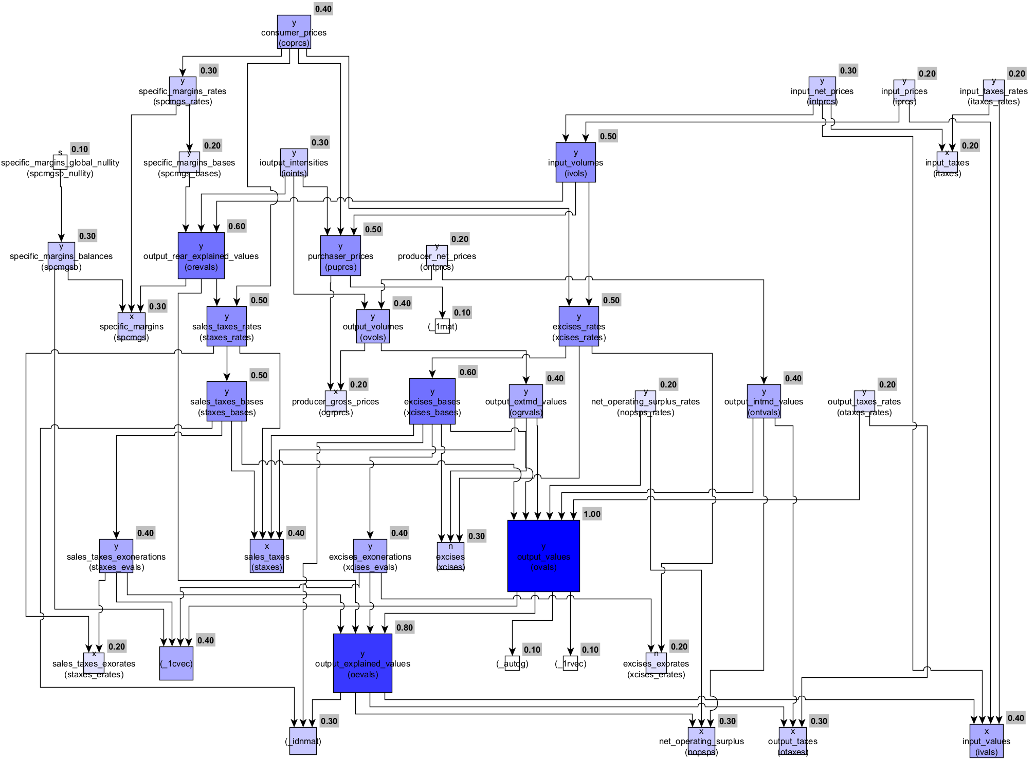
A calibration DAG.

See also

dag_sorter().

property _dag_items(self)

DAG-destined itemized version of _arrays_mdata.

property dag_resolved_callables(self)

Instance-cached property version of _dag_resolver().

Example

>>> idag  = (s := MSystem()).dag_resolved_callables[0]
>>> names = sorted(
...     s._arrays_mdata[k]['n'] for k, _ in idag
... )
>>> for n in names:  
...     print(n)
_0E1
 ...
_1E32
 ...
added_values
 ...
deflators_sq_lfisher
 ...
excises_premia
 ...
zeros_vector_transpose

property _œvars_names(self)

Optimization scaling variables’ private names.

Note

This attribute is not intended to be used publicly.

Example

>>> s = MSystem(
...     'examples/ut(KLEM-BRICS-202006)@sol.xlsx', {
...         'mappings'                 : 'entities',
...         'input_volumes'            : 'i-vols',
...         'input_values'             : 'i-vals',
...         'contrib_taxes'            : 'c-txs',
...         'producer_gross_prices'    : 'av-p-prices',
...         'consumer_prices'          : 'c-prices',
...         'output_volumes'           : 'o-vols',
...         'excises_totals'           : 'exs-tot',
...         'sales_taxes_totals'       : 's-txs-tot',
...         'sales_taxes_exorates'     : '¬%(s-txs)',
...         'specific_margins'         : 'sp-mgs',
...         'unemployment_rates'       : 'u-rates',
...         'unemployment_rates_shoptr': 'η(u-rates)',
...         'available_volumes_grates' : 'δ(caps)',
...         'available_volumes_drates' : 'θ(caps)',
...     }
... )
>>> s._œvars_names  
['_lsag_o', ...]

_hvars_getter(self, Ωs: (list|tuple)[Callable] = (), names_only: bool = False)

Dictionary of the arrays to be mobilized by code_objects_getter.

Parameters

• Ωs (tuple[Callable]) – Systems whose signature is to be inspected so as to determine the list of (keyword only) arguments to be kept. To () by default, which boils down to keeping all arrays.

• names_only (bool) – Whether arrays are to be put aside. Set to False by default.

Note

This method is not intended to be used publicly.

property _hvars_names(self)

List of the parameters’ names to be mobilized by code_objects_getter.

Note

This method is not intended to be used publicly.

Example

>>> s = MSystem(
...     'examples/ut(KLEM-BRICS-202006)@sol.xlsx', {
...         'mappings'                 : 'entities',
...         'input_volumes'            : 'i-vols',
...         'input_values'             : 'i-vals',
...         'contrib_taxes'            : 'c-txs',
...         'producer_gross_prices'    : 'av-p-prices',
...         'consumer_prices'          : 'c-prices',
...         'output_volumes'           : 'o-vols',
...         'excises_totals'           : 'exs-tot',
...         'sales_taxes_totals'       : 's-txs-tot',
...         'sales_taxes_exorates'     : '¬%(s-txs)',
...         'specific_margins'         : 'sp-mgs',
...         'unemployment_rates'       : 'u-rates',
...         'unemployment_rates_shoptr': 'η(u-rates)',
...         'available_volumes_grates' : 'δ(caps)',
...         'available_volumes_drates' : 'θ(caps)',
...     }
... )
>>> s._hvars_names  
['_ivals', '_spcmgs', ..., '_xa1']

See also

_hvars_getter().

_type_duct_expander(self, ለ: Callable, _qn_: str = __qualname__)

Dynamically injects a new functional outflow into the class blueprint.

Parameters

• ለ (Callable) – The function to be bound as staticmethod.

• _qn_ (str) – Private argument assigned at the class level.

_compose_chain(self, sheet_key: str)

Recursively collapses a nested symbolic composition into its terminal form.

Parameters

sheet_key (str) – Internal key of the composition to be processed.

property _constraints_reachability_map(self)

Sparse boolean-alike reachability maps between exogenous variables and constraints ([c]) as well as between exogenous variables themselves ([x]).

Note

Unknown and known exogenands are represented by 𝒳 and α respectively.

Example

>>> _ld, MSystem._lifted_dag = MSystem._lifted_dag, True
>>> df = MSystem(
...     'examples/ut(KLEM-BRICS-202006).xlsx', dict(
...         input_volumes            = 'i-vols',
...         input_values             = 'i-vals',
...         producer_gross_prices    = 'av-p-prices',
...         consumer_prices          = 'c-prices',
...         output_volumes           = 'o-vols',
...         ordinal_volumes          = 'w-vols',
...         contrib_taxes            = 'c-txs',
...         markets_rents            = 'nos',
...         sales_taxes_totals       = 's-txs-tot',
...         sales_taxes_exorates     = '¬%(s-txs)',
...         specific_margins         = 'sp-mgs',
...         available_volumes_grates = 'δ(caps)',
...         available_volumes_drates = 'θ(caps)',
...         income_private_circuit   = 'inc-circuit',
...         mappings                 = 'entities',
...     )
... )._constraints_reachability_map
>>> df.T
                                [c]
                            _ovols¹
                         ogrprcs_ˉ¹
                             _ovols
                                  *
                                  *
                                  *
                                  n
                                  a    z
                                  o e_kl e_kle o_kl o_kle
ogrprcs_ * * * n a o              α    .     .    .     .
                 z e_kl           .    𝒳     .    .     .
                   e_kle          .    .     𝒳    .     .
                   o_kl           .    .     .    𝒳     .
                   o_kle          .    .     .    .     𝒳
>>> MSystem._lifted_dag = _ld

property _ŕmaps(self)

Reachabilities between 1) constraints and their exogenous fibers and 2) between fibers themselves.

Examples

>>> _ld, MSystem._lifted_dag = MSystem._lifted_dag, True
>>> s = MSystem(
...     'examples/ut(KLEM-BRICS-202006).xlsx', dict(
...         input_volumes            = 'i-vols',
...         input_values             = 'i-vals',
...         producer_gross_prices    = 'av-p-prices',
...         consumer_prices          = 'c-prices',
...         output_volumes           = 'o-vols',
...         ordinal_volumes          = 'w-vols',
...         contrib_taxes            = 'c-txs',
...         markets_rents            = 'nos',
...         sales_taxes_totals       = 's-txs-tot',
...         sales_taxes_exorates     = '¬%(s-txs)',
...         specific_margins         = 'sp-mgs',
...         available_volumes_grates = 'δ(caps)',
...         available_volumes_drates = 'θ(caps)',
...         income_private_circuit   = 'inc-circuit',
...         mappings                 = 'entities',
...     )
... )
>>> s._ŕmaps  
{'c': {('[c]', '_ovols¹', 'ogrprcs_ˉ¹', '_ovols', (0, 2)): ...}
>>> MSystem._lifted_dag = _ld

property _mmaps(self)

Upstream reflection of the point-like positions of the data being subject to (static) constraints under multiple perspectives.

Note

This method is not intended to be used publicly.

See also

_xmaps().

property _xmaps(self)

Point-like data-space positions of optimizers.

Note

This method is not intended to be used publicly.

See also

_x́maps() and _x̀maps().

_x́maps(self)

_mmaps-tempered version of _xmaps, i.e. symbolically solved unknowns.

Note

This method is not intended to be used publicly.

See also

_xmaps() and _x̀maps().

_x̀maps(self)

_mmaps-tempered complement of _x́maps, i.e. still numerically solved unknowns.

Note

This method is not intended to be used publicly.

See also

_x́maps() and _xmaps().

_set_xlanes(self, _ppath: str = PACHEDIR)

Set the equation system’s working environment.

Parameters

_ppath (str) – Private argument assigned at the class level.

See also

_set_xmains()’s note.

property _symbolization_gain(self)

Indicate whether and how symbolic rearrangement is beneficial in terms of space complexity.

Example

>>> MSystem()._symbolization_gain
(None, 0.0)

>>> _ld, MSystem._lifted_dag = MSystem._lifted_dag, True
>>> MSystem(
...     'examples/ut(KLEM-BRICS-202006).xlsx', dict(
...         input_volumes            = 'i-vols',
...         input_values             = 'i-vals',
...         producer_gross_prices    = 'av-p-prices',
...         consumer_prices          = 'c-prices',
...         output_volumes           = 'o-vols',
...         ordinal_volumes          = 'w-vols',
...         contrib_taxes            = 'c-txs',
...         markets_rents            = 'nos',
...         sales_taxes_totals       = 's-txs-tot',
...         sales_taxes_exorates     = '¬%(s-txs)',
...         specific_margins         = 'sp-mgs',
...         available_volumes_grates = 'δ(caps)',
...         available_volumes_drates = 'θ(caps)',
...         income_private_circuit   = 'inc-circuit',
...         mappings                 = 'entities',
...     )
... )._symbolization_gain
(True, 0.3076923076923077)
>>> MSystem._lifted_dag = _ld

property code_objects_getter(self)

Return a partial version of _code_objects_getter() (private and undocumented) responsible for dynamically generating a JAX-friendly dependency-resolved instance-method specifically related to the model calibration and recursions, with a mean squared error or sum of squares scalar objective.

Note

The state of this property attribute directly depends on _dag_items’s. Anyway, this method is not intended to be used publicly.

Example

>>> s = MSystem(
...     'examples/ut(KLEM-BRICS-202006)@sol.xlsx', {
...         'mappings'                 : 'entities',
...         'input_volumes'            : 'i-vols',
...         'input_values'             : 'i-vals',
...         'contrib_taxes'            : 'c-txs',
...         'producer_gross_prices'    : 'av-p-prices',
...         'consumer_prices'          : 'c-prices',
...         'output_volumes'           : 'o-vols',
...         'excises_totals'           : 'exs-tot',
...         'sales_taxes_totals'       : 's-txs-tot',
...         'sales_taxes_exorates'     : '¬%(s-txs)',
...         'specific_margins'         : 'sp-mgs',
...         'unemployment_rates'       : 'u-rates',
...         'unemployment_rates_shoptr': 'η(u-rates)',
...         'available_volumes_grates' : 'δ(caps)',
...         'available_volumes_drates' : 'θ(caps)',
...     }
... )
>>> d = s.code_objects_getter()
>>> d['script']  
<code object <module> at ..., file "<string ''>", ...>
>>> d['repr']()  
...

_definjecter(self, script, /, fname: str)

Models definer.

Parameters

• script (types.CodeType) – Modeled system’s compiled script.

• fname (str) – Modeled system’s underlying function’s name.

Note

This method is not intended to be used publicly.

property _proc_cmds(self)

Processed commands, originally found in file via the CUNK_0D_SYM, RUNK_0D_SYM and RUNK_1D_SYM symbols.

Note

This method filters out commands not being located onto _localizations.

Example

>>> s0 = MSystem(
...     'examples/ut(KLEM-BRICS-202006).xlsx', dict(
...         producer_gross_prices='av-p-prices'
...     )
... )
>>> s0._proc_cmds  
{'C': ({'ogrprcs_': {(2010,): (0, ...)}}, ...), 'R': ...}

Keeping the above note in mind, no recursion commands, i.e. RUNK_0D_SYM and RUNK_1D_SYM, are shown. While the sheet 'av-p-prices' contains some of them, it does so through the excel notes, not explicitly associated to any specific (time) localization. Let’s instantiate another MSystem with a sheet that explicite an entire _localizations.

>>> MSystem(
...     'examples/ut(KLEM-BRICS-202006).xlsx', {
...         'consumer_prices': 'c-prices',
...         **s0._sheets_names,
...     },
... )._proc_cmds  
{'C': ({'ogrprcs_': {(2010,): (0, ...)}}, ...), 'R': ...}

property wbook_specs(self)

_ilocalization-variant work book specificities such as the declared calibration’s unknowns, their number, etc.

Example

Let’s load a lot of tables for the sake of this example.

>>> s = MSystem(
...     'examples/ut(KLEM-BRICS-202006)@sol.xlsx', dict(
...         input_values          = 'i-vals',
...         contrib_taxes         = 'c-txs',
...         producer_gross_prices = 'av-p-prices',
...         sales_taxes_totals    = 's-txs-tot',
...         sales_taxes_exorates  = '¬%(s-txs)',
...         specific_margins      = 'sp-mgs',
...     )
... )
>>> s._utils.otbprint(s.wbook_specs['public'])
{
  "graph_options": {
    "detailed_excises": false,
    "detailed_sales_taxes": false,
    "detailed_trade_margins": true,
    "exogenous_market_rents": true,
    "reflected_rights": false,
    "relative_contrib_taxes": false,
    "relative_market_rents": false,
    "relative_other_costs": false,
    "relative_sales_taxes": false,
    "relative_trade_margins": false
  },
  "resolution_options": {
    "aggregated_constraints": true,
    "autodiffed_hessian": false,
    "autodiffed_jacobian": false,
    "averaged_losses": false,
    "broadest_graph": true,
    "compiled_rcomps": false,
    "complex_underliers": true,
    "cscalingf_logbase": 2.0,
    "densified_arrays": true,
    "hoisted_indexers": true,
    "jitted_derivatives": true,
    "jitted_objective": true,
    "lifted_dag": false,
    "losses_exponent": 2.0,
    "losses_factor": 1.0,
    "nonlinear_decision": false,
    "regressed_iguess": true,
    "regressed_scaling": true,
    "scaled_decision": true,
    "serialized_results": false,
    "unclustered_udms": true,
    "vectorized_udcs": false,
    "without_inequality": false
  },
  "resolution_stats": {
    "dimensionality": 0,
    "solved": false
  }
}

Indeed, nowhere in 'examples/ut(KLEM-BRICS-202006)@sol.xlsx' a cell has ?(t=0) for value, which is the symbol to be used (by default, cf CUNK_0D_SYM) to tell the calibration solver where its unknowns are located within the data space.

Let’s have a look at (one of) the “private” items, keyed by 'unks'.

>>> unks = s.wbook_specs['private']['unks']
>>> s._utils.otbprint(unks.pop('_žλ') and unks)
{
  "__k": [],
  "__s": [],
  "_dim": 0,
  "_x̃s₀": [
    []
  ],
  "_x̃s₁": [
    []
  ],
  "_x̃s₂": [
    []
  ],
  "_z_": [],
  "_ẕ_": []
}

We are confronted to the “null” case for the just-mentioned reason.

__repr__(self)

Instance’s formal string representation.

Example

>>> MSystem(
...     'examples/ut(KLEM-BRICS-202006)@sol.xlsx',
...     dict(input_values='i-vals'),
... )
{
  "graph_options": {
    "detailed_excises": False,
    "detailed_sales_taxes": False,
    "detailed_trade_margins": True,
    "exogenous_market_rents": True,
    "reflected_rights": False,
    "relative_contrib_taxes": False,
    "relative_market_rents": False,
    "relative_other_costs": False,
    "relative_sales_taxes": False,
    "relative_trade_margins": False
  },
  "resolution_options": {
    "aggregated_constraints": True,
    "autodiffed_hessian": False,
    "autodiffed_jacobian": False,
    "averaged_losses": False,
    "broadest_graph": True,
    "compiled_rcomps": False,
    "complex_underliers": True,
    "cscalingf_logbase": 2.0,
    "densified_arrays": True,
    "hoisted_indexers": True,
    "jitted_derivatives": True,
    "jitted_objective": True,
    "lifted_dag": False,
    "losses_exponent": 2.0,
    "losses_factor": 1.0,
    "nonlinear_decision": False,
    "regressed_iguess": True,
    "regressed_scaling": True,
    "scaled_decision": True,
    "serialized_results": False,
    "unclustered_udms": True,
    "vectorized_udcs": False,
    "without_inequality": False
  },
  "resolution_stats": {
    "dimensionality": 0,
    "solved": False
  }
}

classmethod _lfancy_substracter(cls, lfancys: list[tuple[type], tuple[int, tuple[tuple[int]]]], nfancy: (tuple|list)[tuple[int]], ref_iloc: int = None)

Subtract a numpy-friendly fancy index from a per-localization (onto _localizations) counterpart.

Parameters

• lfancys (tuple) – Sequence of (localized) indexes to be processed.

• nfancy (tuple or list) – Unique (non-localized) fully specified advanced index to be subtracted from lfancys.

• ref_iloc (int) – _ilocalization to be used as reference for filtering. Set to None by default.

:Example

>>> MSystem._lfancy_substracter(
...     nfancy=[(0, 0, 1), (1, 1, 1), (1, 2, 3)],
...     lfancys=[
...         (('a',), (0, (1, 1, 1, 2), (1, 2, 3, 3))),
...         (('b',), (1, (1, 1, 1), (1, 2, 3))),
...     ],
... )
[(('a',), (0, (1, 2), (3, 3))), (('b',), (1, (1, 1), (1, 2)))]

>>> MSystem._lfancy_substracter(
...     ref_iloc=0, nfancy=[(0, 0, 1), (1, 1, 1), (1, 2, 3)],
...     lfancys=[
...         (('a',), (0, (1, 1, 1, 2), (1, 2, 3, 3))),
...         (('b',), (1, (1, 1, 1), (1, 2, 3))),
...     ],
... )
[(('a',), (0, (1, 2), (3, 3))), (('b',), (1, (1,), (3,)))]

>>> MSystem._lfancy_substracter(
...     ref_iloc=0, nfancy=[(0, 0, 0), (1, 1, 1), (1, 2, 3)],
...     lfancys=[
...         (('a',), (0, (1, 1, 1, 2), (1, 2, 3, 3))),
...         (('b',), (1, (1, 1, 1), (1, 2, 3))),
...     ],
... )
[(('a',), (0, (2,), (3,))), (('b',), (1, (), ()))]

classmethod _lfancy_merger(cls, lfancys: list[tuple[type], tuple[int, tuple[tuple[int]]]], _otyper: Callable = lambda s: sorted(set(s)))

Merge localized numpy-friendly fancy indexes on a per-localization basis (onto _localizations).

Parameters

• lfancys (tuple) – Sequence of (localized) indexes to be processed.

• _otyper (Callable) – Private argument assigned at the class level. To lambda s: sorted(set(s)).

Example

>>> a, b = MSystem._lfancy_merger(
...     lfancys=[
...         (('a',), (0, (1, 1, 1), (1, 2, 3))),
...         (('b',), (1, (1, 1, 1), (1, 2, 3))),
...         (('a',), (0, (1, 1, 2), (1, 2, 3))),
...     ]
... )
>>> a
(('a',), (0, (1, 1, 1, 2), (1, 2, 3, 3)))
>>> b
(('b',), (1, (1, 1, 1), (1, 2, 3)))

property uid(self)

Solver-specialized version of uid.

Note

This attribute is session-stable and cross-platform.

Example

>>> MSystem().uid
'mrwJyYTo4Hh0'

_iguess_specifier(self, xmaps: dict[str, list[tuple[int]]], _xuign: str = XUNK_IG_CNAME, **_kws: 'np.ndarray|bool')

Specify the initial position of the system in the decision-space.

Parameters

• xmaps (dict) – Point-like data-space positions of optimizers, (such as _xmaps).

• _xuign (str) – Private argument assigned at the class level. Set to XUNK_IG_CNAME.

• **_kws (numpy.ndarray or bool) – Private keyword arguments, if any.

Note

This method is not intended to be used publicly.

_optim_specifier(self, iguess: np.ndarray = None, _xuign: str = XUNK_IG_CNAME, _xusfn: str = XUNK_SF_CNAME)

Define a set of (callable) specifiers related to a given optimization process, such as initial guesses, scaling factors, variables’ bounds, etc.

Parameters

• iguess (numpy.ndarray) – Initial guess the solver should be forced to start from. Set to None by default, i.e. inferred/taken from the numerical context.

• _xuign (str) – Private argument assigned at the class level. Set to XUNK_IG_CNAME.

• _xusfn (str) – Idem. Set to XUNK_SF_CNAME.

Note

This method is not intended to be used publicly.

_jacobian_c_renormer(self, ῼs: (tuple|list)[Callable], **_kws: float)

Compute the scaling factors associated to the decision components of the system of interest.

Parameters

• ῼs (tuple or list) – Z-systems of interest.

• **_kws (float) – Private keyword arguments, if any.

_scale_inferrer(self, **_kws: float)

Scale a vector decision variable using the Ruiz equilibration algorithm.

Parameters

**_kws (float) – Private keyword arguments, if any.

_scale_explorer(self, sheet_id: str, _ia: int = 0)

Explore attributes’ companions for an exploitable base scale.

Parameters

• sheet_id (str) – Public or internal/private name of the worksheet to be processed.

• _ia (int) – Private argument used for recursion purpose.

Note

This method is not intended to be used publicly.

Example

>>> sheet_name = 'sp-mgs'
>>> s = MSystem(
...     'examples/ut(KLEM-BRICS-202006)@sol.xlsx', dict(
...         input_values='i-vals',
...         contrib_taxes='c-txs',
...         specific_margins=sheet_name,
...     )
... )
>>> s._scale_explorer(sheet_name).item()
115326071.17840433

classmethod _distributor_blueprint(cls, x, /, z: np.ndarray, ẕ: np.ndarray, k: np.ndarray, s: np.ndarray, μ: np.ndarray, arrays: dict[str, np.ndarray], χ: int, dγ: float, Ѡs: tuple[Callable], žλ: Callable, ᴧs: tuple[tuple[str, type]], λs: dict[str, Callable], ʈs: dict[str, tuple], keỳs: tuple[str], yćḿs: tuple[tuple[str, str, tuple[str, tuple[int]]]], śłćs: tuple[tuple[str, tupe[str, tuple[int]]]], slcs: tuple[str, tuple[str, tuple[int]]], full_output: bool, *, Ω: Callable, **_kῶs: np.ndarray)

Wrapper responsible for distributing the solver’s unknowns among the (modeled) system’s exogenous arrays.

Parameters

• x (numpy.ndarray) – Array of real elements everted during minimization.

• z (numpy.ndarray) – x’s first scaling parameter.

• ẕ (numpy.ndarray) – x’s second scaling parameter.

• k (numpy.ndarray) – x’s jacobian columns scaling parameter.

• s (numpy.ndarray) – x’s group level multiplier on the target column-norm level used to solve for k.

• µ (numpy.ndarray) – Levenberg-Marquardt damping parameter.

• arrays (dict) – Dictionary of arrays constitutive of the modeled system.

• χ (int) – Archetype of _χ.

• dγ (float) – Archetype of _dγ.

• Ѡs (tuple) – Sequence of symbolically defined Ω’s simplifiers.

• žλ (Callable) – x’s scaler.

• ᴧs (tuple) – Archetype of _ᴧs (undocumented).

• λs (dict) – Archetype of _λs (undocumented).

• ʈs (dict) – Archetype of _ʈs (undocumented).

• keỳs (tuple) – Sequence of arrays’ names to be mobilized by Ѡs’s elements.

• yćḿs (tuple) – Bunch of key materials processed for knowns injection.

• śłćs (tuple) – Bunch of key-slice materials processed for knowns extraction.

• slcs (tuple) – Bunch of key-slice materials processed for unknowns injection.

• full_output (bool) – Whether all intermediary objects are to be returned as well as the primary quantity of interest, that is the grand_saturation of the system at χ.

• Ω (Callable) – System of interest.

• **_kῶs (numpy.ndarray) – Ω-specific keyword arguments.

classmethod _jx_jit(cls, j: bool, copts: dict[str, type] = None, _v_: tuple[str] = (*jx.__version__.split('.'), ))

Either return jax.jit or an identity function.

Parameters

• j (bool) – Whether jax.jit has to be returned.

• copts (dict) – Compilation options argument, for passing to XLA. Set to None by default.

_distributor(self, Ω, /)

Factory method responsible for JAX-JITing the operationalized version of _distributor_blueprint().

Parameters

Ω (Callable) – System of interest.

Important

This method returns an unjitted callable for JITTED_OBJECTIVE set to False.

Note

The arguments of the returned callable are x, z, ẕ, µ, arrays, χ, dγ, žλ, ᴧs, λs, ʈs, slcs and full_output. For details, see _distributor_blueprint().

Example

>>> s = MSystem()
>>> s._distributor(s._xmains_0).__name__
'_cmains_0'

_distributors_fuzzer(self, Ωs, /, fuzzkey: str = '_x̃s₂', **_kws: type)

Evaluate the systems of interest’s (combined) system-specific objective at multiple locations in the decision space.

Parameters

• Ωs (list or tuple) – Systems of interest.

• fuzzkey (str) – Key associated to the sequence of positions in the decision space over which the fuzzing process must be performed. Undocumented for now, options are '_x̃s₀', '_x̃s₁', '_x̃s₂' or '_x̃s₃'. Set to '_x̃s₂' by default.

• **_kws (type) – Private keyword arguments, if any.

Example

>>> s = MSystem()
>>> s._distributors_fuzzer(
...     s._xmain_eqs + s._xmain_ins
... )
[Array([0.], dtype=float64), Array([[0.]], dtype=float64)]

_distributor_jacobian(self, Ω, /)

JAX-JIT-compiled jacobian computer of _distributor.

Parameters

Ω (Callable) – System of interest.

Important

This method returns an unjitted callable for JITTED_DERIVATIVES set to False.

See also

_distributor().

Example

>>> s = MSystem()
>>> s._distributor_jacobian(s._xmains_0).__name__
'_cmains_0_jac'

_soberly_computed(self, ncond: bool|int = False)

Control-flow performatively stating whether downstream callable derivatives’ definition do not imply full (and costly) computations.

Parameters

ncond (bool or int) – Boolean specifying whether the value of the attribute _aggregated_constraints is to be considered as a (necessary) condition favoring full computation. Set to False by default.

See also

AGGREGATED_CONSTRAINTS.

Note

This method’s tradeoff is based on the decision’s dimensionality and (undocumented private) class’s attributes such as _batch_size and _forced_lnrzd.

Example

>>> m = MSystem(
...     'examples/ut(KLEM-BRICS-202006).xlsx', sheets_names={
...         'producer_gross_prices': 'av-p-prices',
...         'input_values'         : 'i-vals',
...     }
... )
>>> m.wbook_specs['public']['resolution_stats']['dimensionality']
9
>>> m._batch_size
100000
>>> m._forced_lnrzd
False
>>> m._aggregated_constraints
True

>>> m._soberly_computed()
False
>>> m._soberly_computed(ncond=True)
False

>>> MSystem._batch_size = 8
>>> m._soberly_computed()
{'d': 9, 's': 8}
>>> m._soberly_computed(ncond=True)
False

>>> MSystem._batch_size = 100

_distributor_jacobianl(self, Ω, /)

JAX-JIT-compiled jacobian computer of _distributor based on jvp, i.e. the linearization of the \(0\)th order derivative.

Parameters

Ω (Callable) – System of interest.

Important

This method returns an unjitted callable for JITTED_DERIVATIVES set to False.

See also

_distributor().

Example

>>> s = MSystem()
>>> s._distributor_jacobianl(s._xmains_0).__name__
'_cmains_0_jac'

>>> MSystem._forced_lnrzd = True
>>> s._distributor_jacobianl(
...     s._xmains_0
... ).__name__  
Traceback (most recent call last):
 ...
RuntimeError: ... not allowed.

>>> MSystem._forced_lnrzd = False

_distributor_jacobianls_structurer(self, Ωs, /)

Determine the combined jacobians sparsity pattern of the systems of interest.

Parameters

Ωs (list or tuple) – Systems of interest.

Example

>>> s = MSystem()
>>> s._distributor_jacobianls_structurer(
...     s._xmain_eqs + s._xmain_ins
... )
BCOO(uint8[2, 0], nse=0)

_distributor_jacobianls_fuzzer(self, Ωs, /, fuzzkey: str = '_x̃s₂', sparse: bool = False, **_kws: type)

Evaluate the systems of interest’s (combined) system-specific jacobian at multiple locations in the decision space.

Parameters

• Ωs (list or tuple) – Systems of interest.

• fuzzkey (str) – Key associated to the sequence of positions in the decision space over which the fuzzing process must be performed. Undocumented for now, options are '_x̃s₀', '_x̃s₁', '_x̃s₂' or '_x̃s₃'. Set to '_x̃s₂' by default.

• sparse (bool) – Whether the evaluation should resort to sparse methods and objects. To False by default.

• **_kws (type) – Private keyword arguments, if any.

Note

In the sparse=False case, this method raises an error if a NaN is detected in any of the computed jacobians.

Example

>>> s = MSystem()
>>> s._distributor_jacobianls_fuzzer(
...     s._xmain_eqs + s._xmain_ins
... )  
[Array([], shape=(1, 0), dtype=float64), ...]

_distributor_sp_jacobianl(self, Ω, /)

JAX-JIT-compiled sparse jacobian computer of _distributor.

Note

This method can only differentiate functions whose output is exactly 1-dimensional.

Parameters

Ω (Callable) – System of interest.

Important

This method returns an unjitted callable for JITTED_DERIVATIVES set to False.

See also

_distributor()., _distributor_jacobianls_structurer().

Example

>>> s = MSystem()
>>> s._distributor_sp_jacobianl(s._xmains_0).__name__
'_cmains_0_jacl_sp'

_distributor_hessian(self, Ω, /)

JAX-JIT-compiled hessian computer of _distributor.

Parameters

Ω (Callable) – System of interest.

Important

This method returns an unjitted callable for JITTED_DERIVATIVES set to False.

See also

_distributor().

Example

>>> s = MSystem()
>>> s._distributor_hessian(s._xmains_0).__name__
'_cmains_0_hess'

_distributor_hessianl(self, Ω, /)

JAX-JIT-compiled hessian computer of _distributor based on hvp, i.e. the linearization of the localized Jacobian.

Parameters

Ω (Callable) – System of interest.

Important

This method returns an unjitted callable for JITTED_DERIVATIVES set to False.

See also

_distributor().

Example

>>> s = MSystem()
>>> s._distributor_hessianl(s._xmains_0).__name__
'_cmains_0_hess'

>>> MSystem._forced_lnrzd = True
>>> s._distributor_hessianl(
...     s._xmains_0
... ).__name__  
Traceback (most recent call last):
 ...
RuntimeError: ... not allowed.

>>> MSystem._forced_lnrzd = False

_distributor_hessianl_lws(self, Ω, /)

JAX-JIT-compiled hessian Lagrangian weighted sum computer of _distributor.

Parameters

Ω (Callable) – System of interest.

Important

This method returns an unjitted callable for JITTED_DERIVATIVES set to False.

See also

_distributor().

Attention

This method is about to be removed since implying very inefficient objects formulation.

Example

>>> s = MSystem()
>>> s._distributor_hessianl_lws(s._xmains_0).__name__
'_cmains_0_hessl_lws'

_distributor_hessianls_structurer(self, Ωs, /, **_kws: type)

Determine the combined hessians sparsity pattern of the systems of interest.

Parameters

• Ωs (list or tuple) – Systems of interest.

• **_kws (type) – Private keyword arguments, if any.

Example

>>> s = MSystem(
...     'examples/ut(KLEM-BRICS-202006).xlsx', dict(
...         input_volumes            = 'i-vols',
...         input_values             = 'i-vals',
...         producer_gross_prices    = 'av-p-prices',
...         consumer_prices          = 'c-prices',
...         output_volumes           = 'o-vols',
...         ordinal_volumes          = 'w-vols',
...         contrib_taxes            = 'c-txs',
...         markets_rents            = 'nos',
...         sales_taxes_totals       = 's-txs-tot',
...         sales_taxes_exorates     = '¬%(s-txs)',
...         specific_margins         = 'sp-mgs',
...         available_volumes_grates = 'δ(caps)',
...         available_volumes_drates = 'θ(caps)',
...         income_private_circuit   = 'inc-circuit',
...         mappings                 = 'entities',
...     )
... )
>>> s._distributor_hessianls_structurer(
...     s._xmain_obs[:1] + s._xmain_eqs + s._xmain_ins
... )
BCOO(uint8[13, 13], nse=81)

_distributor_sp_hessianl(self, Ω, /)

JAX-JIT-compiled sparse hessian computer of _distributor.

Note

This method can only differentiate functions whose output is exactly 1-dimensional.

Parameters

Ω (Callable) – System of interest.

Important

This method returns an unjitted callable for JITTED_DERIVATIVES set to False.

See also

_distributor(), _distributor_sp_jacobianl(), _distributor_hessianls_structurer().

Example

>>> s = MSystem()
>>> s._distributor_sp_hessianl(
...     s._xmains_0
... ).__name__  
'_cmains_0_hessl_sp'

_distributor_derivatives(self, Ω, /)

Tuple-gather the callables returned by _distributor(), _distributor_jacobian(), _distributor_jacobianl(), _distributor_hessian(), _distributor_hessianl(), and _distributor_hessianl_lws() in this very order, when evaluated at Ω.

Parameters

Ω (Callable) – System of interest.

See also

_distributor().

_distributor_decomposer(self, Ω: Callable, order: int = 0, relative: bool = False, fuzzed: bool = True, fuzzkey: str = None, aggregator: Callable = ft.partial(np.mean, axis=0), as_frame: bool = True, set_œscalers: str = 'restored', full_output: bool = False, _usym: str = UNIV_SYM, **_kws: type)

Compute the components’ zeroth or first order contributions to the total system-specific function of interest.

Parameters

• Ω (Callable) – System of interest.

• order (int) – Differentiation order, ranging from 0 to 1. Set to 0 by default.

• relative (bool) – Whether the contributions should be returned as summing-to-one shares. Set to False by default.

• fuzzed (bool) – Whether the contributions must be evaluated at multiple locations in the decision space. Set to True by default.

• fuzzkey (str) – Key associated to the sequence of positions in the decision space over which the fuzzing process must be performed. Undocumented for now, options are '_x̃s₀', '_x̃s₁', '_x̃s₂' or '_x̃s₃'. Set to None by default, which actually boils down to '_x̃s₁' when fuzzed and '_x̃s₀' otherwise.

• aggregator (Callable) – Aggregating function to be used over the contributions being fuzzed. Set to 0th-axis-partialized numpy.mean by default, which is neutral for fuzzed=False.

• as_frame (bool) – Whether the result is to be returned as pandas.DataFrame. Set to True by default.

• set_œscalers (str) – Option specifying whether, once the contributions are computed, scalers can either be 'restored', 'reset' or 'left_as_is' as is. Indeed, this method set all optimization scalers to 1 prior to performing its calculations. Set to 'restored' by default.

• full_output (bool) – Whether the intermediary total Ω-derived jacobian should be returned as well, incidentally aimlessly calculated as relative=False. Set to False by default.

• _usym (str) – Unaccessible argument defined at the class level. Set to UNIV_SYM.

• **_kws (type) – Private keyword arguments, if any.

_set_œscalers(self, value: float = 1.0, withheld: (tuple|list)[str] = None, discarded: (tuple|list)[str] = None)

Gather and identically update all optimization scalers.

Parameters

• value (float) – Value the arrays must be updated to. Set to 1. by default.

• withheld (list or tuple) – Sequence of scalers to be updated. Set to None by default, i.e. no scaler is put aside.

• discarded (list or tuple) – Sequence of scalers not to be updated. Set to None by default, i.e. no scaler is put aside.

Note

This method returns self for the sake of chaining.

_compute_opscalers(self, ῼs: (tuple|list)[Callable], method: str|tuple[str, dict[str, type]], **_kws: type)

Compute the scaling factors associated to the optimization components (such as the objective and constraints) of the system of interest.

Parameters

• ῼs (tuple or list) – Z-systems of interest.

• method (str or tuple) – Method by which scale factors are calculated, among 'jacobian-based', 'curvature-based' and 'none'. This argument can also be provided as 2-uple whose second component consists in a parameterizing (undocumented) dict.

• **_kws (type) – Private keyword arguments, if any.

Note

1. ATM, the method 'jacobian-based' can only be used over (ῼs-contained) systems that have the exact same components and whose derived function are scalar valued, otherwise, an error is raised.

2. This method returns self for the sake of chaining.

3. This method is not intended to be used publicly.

_systems_interpreter(self, Ὦs: (tuple|list)[Callable], order: int = 0, with_ƨnames: bool = False, unjitted: bool = True)

Conceive and return the systems-specific partialized functions of interest.

Parameters

• Ὦs (tuple or list) – Any-tribe systems of interest.

• order (int) – Differentiation order, ranging from 0 to 2, with the latter two being untested. Set to 0 by default.

• with_ƨnames (bool) – Whether the returned callables should be “zipped” with their corresponding system’s ~._ƨnames attribute. Set to False by default.

• unjitted (bool) – Whether the returned functions have to be unjitted. To True by default.

Note

This method (whose underliers are unjitted) is not intended to be used publicly.

_zsystems_evaluator(self, ῼs: (tuple|list)[Callable], order: int = 0, fuzzed: bool = True)

Evaluate the \(n\)th order derivative of the Z-systems-specific functions of interest.

Parameters

• ῼs (tuple or list) – Z-systems of interest.

• order (int) – Derivation order passed to _systems_interpreter(). Set to 0 by default.

• fuzzed (bool) – Whether the contributions must be evaluated at multiple locations in the decision space. Set to True by default.

Note

This method (whose underliers are unjitted) is not intended to be used publicly.

_compute_residuals_grand_mask(self, ῼ, /, _0λ: Callable = __0λ, _hvλ: Callable = __hvλ)

Compute the mask of the callable’s output prior to aggregation, if any.

Parameters

• ῼ (Callable) – Z-system of interest.

• _0λ (Callable) – Private argument assigned at the class level. Set to lambda _: _.

• _hvλ (Callable) – Idem. Set to lambda o, _λ=opr.itemgetter('h', 'v'): (*map(int, _λ(o)),)

Note

This method is not intended to be used publicly.

_compute_residuals_grand_masks(self, ῼs: (list|tuple)[Callable])

Vectorized version of _compute_residuals_grand_mask().

Parameters

ῼs (list or tuple) – Systems of interest.

Note

This method is not intended to be used publicly.

property _minimization_coargumenter(self)

Return a callable that provides static parameters required by the objective function during optimization.

This method constructs and returns a callable object that, when invoked, supplies the necessary ancillary arguments to the modeling function. These additional parameters might include hyperparameters, configuration settings, or any other data that influences the behavior of the objective function but is not part of the standard argument set.

Note

This method is not intended to be used publicly.

_minimization_jacobian_computer(self, Ω: Callable, as_frame: bool = True)

Compute the gradient of the system-specific function of interest, evaluated at the best possible position within the decision space, depending on whether it is called before or after the minimization has occurred.

Parameters

• Ω (Callable) – System of interest.

• as_frame (bool) – Whether the result is to be returned as pandas.DataFrame. Set to True by default.

See also

minimization_jacobian().

property minimization_jacobian(self)

Attribute storing the gradient of the objective function evaluated at the best possible position within the solution space, depending on whether it is called before or after the minimization has occurred.

When invoked after the minimization, this attribute represents the gradient vector of the objective function at the point where the function attains its minimum value, indicating the rate and direction of change of the function at that point. This can be used to verify optimality conditions or analyze the sensitivity of the solution.

Note

This attribute’s name contains the word “jacobian” instead of “gradient” as a first step toward generalization.

See also

_minimization_jacobian_computer().

Example

>>> sheets_names = {
...     'mappings'                          : 'entities',
...     'income_private_circuit'            : 'inc-circuit',
...     # Cross-sections
...     'input_values'                      : 'i-vals',
...     'unemployment_rates'                : 'u-rates',
...     'unemployment_rates_shoptr'         : 'η(u-rates)',
...     'producer_gross_prices'             : 'av-p-prices',
...     'output_volumes'                    : 'o-vols',
...     'ordinal_volumes'                   : 'w-vols',
...     'markets_rents'                     : 'nos',
...     'contrib_taxes'                     : 'c-txs',
...     'sales_taxes_totals'                : 's-txs-tot',
...     'sales_taxes_exorates'              : '¬%(s-txs)',
...     'excises_totals'                    : 'exs-tot',
...     'specific_margins'                  : 'sp-mgs',
...     'consumer_prices'                   : 'c-prices',
...     # Time series
...     'input_volumes'                     : 'i-vols',
...     # δ
...     'markets_rents_rates_grates'        : 'δ(nos-rates)',
...     'contrib_taxes_rates_grates'        : 'δ(c-txs-rates)',
...     'sales_taxes_totals_rates_grates'   : 'δ(s-txs-tot-rates)',
...     'specific_margins_rates_grates'     : 'δ(sp-mgs-rates)',
...     'consumer_prices_grates'            : 'δ(c-prices)',
...     'unemployment_rates_grates'         : 'δ(u-rates)',
...     'available_volumes_grates'          : 'δ(caps)',
...     'skizo_budgets_shares_grates'       : 'δ(skb-shares)',
...     'input_volumes_grates'              : 'δ(i-vols)',
...     'ioq_intensities_order3_grates'     : 'δ(io-ints-o3)',
...     # θ
...     'available_volumes_drates'          : 'θ(caps)',
...     'ioq_shares_drates'                 : 'θ(io-shas-o1)',
... }
>>> s = MSystem(
...     'examples/ut(KLEM-BRICS-202006).xlsx', sheets_names
... )
>>> s.minimization_jacobian.iloc[:, :-1]
                                    *
                                    *      E₀
                                    𝒵       𝒳 sgn 𝕵       |𝕵|
av-p-prices * * * n a e       (4e+00)  1000.0     -  8.42e-03
                    d e       (4e+00)  1000.0     +  1.28e-33
                      k       (4e+00)  1000.0     +  7.90e-04
                    m e       (4e+00)  1000.0     -  4.00e-03
                    z e_kl    (4e+00)  1000.0     -  4.84e-04
                      e_kle   (4e+00)  1000.0     -  4.40e-04
                      o_kl    (4e+00)  1000.0     -  3.68e-04
                      o_kle   (4e+00)  1000.0     -  3.19e-04
                  w x e       (4e+00)  1000.0     -  0.00e+00
sp-mgs      n a e n d c      ⁺(3e+01)     0.0     -  2.06e-05
                    x e      ⁺(3e+01)     0.0     -  1.32e-04
                    z e_kle  ⁺(3e+01)     0.0     -  2.74e-06
                      o_kle  ⁺(3e+01)     0.0     -  2.99e-06

property _minimization_residuals(self, _usym: str = UNIV_SYM)

Private counterpart of minimization_residuals.

property minimization_residuals(self, _usym: str = UNIV_SYM)

Attribute storing the residuals of the (disaggregated) objective function evaluated at the best possible position within the solution space, depending on whether it is called before or after the minimization has occurred.

Example

>>> sheets_names = {
...     'mappings'                          : 'entities',
...     'income_private_circuit'            : 'inc-circuit',
...     # Cross-sections
...     'input_values'                      : 'i-vals',
...     'unemployment_rates'                : 'u-rates',
...     'unemployment_rates_shoptr'         : 'η(u-rates)',
...     'producer_gross_prices'             : 'av-p-prices',
...     'output_volumes'                    : 'o-vols',
...     'ordinal_volumes'                   : 'w-vols',
...     'markets_rents'                     : 'nos',
...     'contrib_taxes'                     : 'c-txs',
...     'sales_taxes_totals'                : 's-txs-tot',
...     'sales_taxes_exorates'              : '¬%(s-txs)',
...     'excises_totals'                    : 'exs-tot',
...     'specific_margins'                  : 'sp-mgs',
...     'consumer_prices'                   : 'c-prices',
...     # Time series
...     'input_volumes'                     : 'i-vols',
...     # δ
...     'markets_rents_rates_grates'        : 'δ(nos-rates)',
...     'contrib_taxes_rates_grates'        : 'δ(c-txs-rates)',
...     'sales_taxes_totals_rates_grates'   : 'δ(s-txs-tot-rates)',
...     'specific_margins_rates_grates'     : 'δ(sp-mgs-rates)',
...     'consumer_prices_grates'            : 'δ(c-prices)',
...     'unemployment_rates_grates'         : 'δ(u-rates)',
...     'available_volumes_grates'          : 'δ(caps)',
...     'skizo_budgets_shares_grates'       : 'δ(skb-shares)',
...     'input_volumes_grates'              : 'δ(i-vols)',
...     'ioq_intensities_order3_grates'     : 'δ(io-ints-o3)',
...     # θ
...     'available_volumes_drates'          : 'θ(caps)',
...     'ioq_shares_drates'                 : 'θ(io-shas-o1)',
... }
>>> MSystem(
...     'examples/ut(KLEM-BRICS-202006).xlsx', sheets_names
... ).minimization_residuals
                                                   *
                                                   *
                                                   *
                                                   *
                                                   *
                                                   *
                                                   *
A-System _output_volumes       * * * n a o      0.00
                                       z e_kl   0.88
                                         e_kle  0.89
                                         o_kl   0.91
                                         o_kle  0.92
..                                               ...
E-System demand_side_integrity * * * n m o      0.00
                                       z e_kl   0.00
                                         e_kle  0.00
                                         o_kl   0.00
                                         o_kle  0.00

[70 rows x 1 columns]

property _constraints_jacobian(self)

Attribute combining the jacobian of the constraints evaluated at the best possible position within the solution space, depending on whether it is called before or after the minimization has occurred.

Example

>>> sheets_names = {
...     'mappings'                          : 'entities',
...     'income_private_circuit'            : 'inc-circuit',
...     # Cross-sections
...     'input_values'                      : 'i-vals',
...     'unemployment_rates'                : 'u-rates',
...     'unemployment_rates_shoptr'         : 'η(u-rates)',
...     'producer_gross_prices'             : 'av-p-prices',
...     'output_volumes'                    : 'o-vols',
...     'ordinal_volumes'                   : 'w-vols',
...     'markets_rents'                     : 'nos',
...     'contrib_taxes'                     : 'c-txs',
...     'sales_taxes_totals'                : 's-txs-tot',
...     'sales_taxes_exorates'              : '¬%(s-txs)',
...     'excises_totals'                    : 'exs-tot',
...     'specific_margins'                  : 'sp-mgs',
...     'consumer_prices'                   : 'c-prices',
...     # Time series
...     'input_volumes'                     : 'i-vols',
...     # δ
...     'markets_rents_rates_grates'        : 'δ(nos-rates)',
...     'contrib_taxes_rates_grates'        : 'δ(c-txs-rates)',
...     'sales_taxes_totals_rates_grates'   : 'δ(s-txs-tot-rates)',
...     'specific_margins_rates_grates'     : 'δ(sp-mgs-rates)',
...     'consumer_prices_grates'            : 'δ(c-prices)',
...     'unemployment_rates_grates'         : 'δ(u-rates)',
...     'available_volumes_grates'          : 'δ(caps)',
...     'skizo_budgets_shares_grates'       : 'δ(skb-shares)',
...     'input_volumes_grates'              : 'δ(i-vols)',
...     'ioq_intensities_order3_grates'     : 'δ(io-ints-o3)',
...     # θ
...     'available_volumes_drates'          : 'θ(caps)',
...     'ioq_shares_drates'                 : 'θ(io-shas-o1)',
... }
>>> MSystem._aggregated_constraints = False
>>> s = MSystem(
...     'examples/ut(KLEM-BRICS-202006).xlsx', sheets_names
... )
>>> s._constraints_jacobian.loc[
...     :, pd.IndexSlice[:, :, :, :, :, :, 'e']
... ].map("{:.0e}".format).replace('0e+00', '.')
                        av-p-prices                sp-mgs
                                  *                     n
                                  *                     a
                                  *                     e
                                  n             w       n
                                  a  d       m  x       x
                                  e  e       e  e       e
eq_0   * * *  n a e               .  .       .  .       .
                b b          -2e-03  .       .  .       .
                d k               .  .       .  .       .
                  l1         -4e-03  .       .  .  -1e-04
                  o          -1e-03  .       .  .       .
                m *          -2e-03  .       .  .       .
                z e_kl            .  .       .  .       .
                  e_kle           .  .       .  .       .
                  o_kl            .  .       .  .       .
                  o_kle           .  .       .  .       .
       n b b  n m *               .  .  -4e-03  .       .
         d cg n m e               .  .       .  .       .
           e  * * *               .  .       .  .       .
ineq_0 * * *  * * *               .  .       .  .       .
>>> MSystem._aggregated_constraints = True

minimize(self, disp: int = 0, oalgo: str|list[str] = 'sl', salgo: str|tuple[str, dict[str, type]] = 'none', ctypes: tuple[str] = (), rschedule: tuple[float] = (), **soptions: type)

System minimizer.

Parameters

• disp (int) – Control the verbosity of the minimization. Between 0 (nothing is displayed) and 13 (maximal information). Note that values above 4 are inoperative as oalgo is either not 'ip.<>' or not 'sp.<>'. To 0 by default.

• oalgo (str or list) – (Sequence of) optimization(s) method(s). Choices are 'nm' (Nelder Mead), 'cg' (CG), 'jx' (JAX’s BFGS), 'bf' (BFGS), 'lb' (L-BFGS-B), 'tr' (trust-constr), 'nc' ( Newton-CG), 'pw' (Powell), 'sl' (SLSQP), NLOPT’s methods (e.g. 'nl.mma') and IPOPT’s linear solvers (e.g. 'ip.mumps'), as well as the sparse couterparts of the latter (e.g. 'sp.mumps'). To 'sl' by default.

• salgo (str or tuple) – Scaling method to be employed so as to calculate the appropriate objective gradient scale. By default to 'none'. For details, see the documentation regarding _compute_opscalers()’s method argument.

• ctypes (tuple) – Types of constraints to be considered by the optimizer, among 'eq' and 'ineq'. Set to () by default.

• rschedule (tuple or list) – Monotone schedule of target dominance ratios φ between the SSR gradient and the regularizer gradient – with a regularization term à la Levenberg-Marquardt so as to improve numerical conditioning –, used for annealing the regularization strength µ across successive runs. The dominance ratio is \(\phi = \frac{\left\lVert \nabla \mathrm{SSR}(x) \right\rVert_{\infty}}{\left\lVert \nabla R(x) \right\rVert_{\infty}}, \qquad R(x) = \mu \left \lVert x - x_0 \right\rVert_2^2\). Use [np.inf] (or equivalently ()) to disable regularization. Set to () by default.

• **soptions (type) – Algorithm-dependent options.

See also

calibrate(), evolve().

Note

1. 'ip.<>'- and 'sp.<>'-based arguments requires the installation of cyipopt and IPOPT.

2. 'nl'-based oalgos are extremly conservative by defaulting their ftol_abs, ftol_rel, xtol_abs and xtol_rel companion arguments to 0.

_optim_related_stats_formatter(self, arrays: dict[str, np.ndarray], qslices: list[tuple[str, type]])

Pretty-format a bunch of solvers’ statistics.

Parameters

• arrays (dict) – Dictionary of named statistics to be printed.

• qslices (list) – Bunch of name-key-slice materials processed for printing.

Note

This method is not intended to be used publicly.

Example

>>> # ...

classmethod _optim_related_stat_formatter(cls, a: np.ndarray, qslices: list[tuple[str, type]], aname: str = None, dslice: int = None)

Pretty-format a given solvers’ statistic.

Note

This method is not intended to be used publicly.

Parameters

• a (numpy.array) – Array to be processed.

• qslices (list) – Bunch of name-key-slice materials processed for printing.

• aname (str) – Name of a, if any. Set to None by default.

• dslice (int) – Identifying slice’s dimensionality, inferred otherwise. Set to None by default.

calibrate(self, validating: bool = True, **options: type)

Preset property version of minimize().

Parameters

• validating (bool) – Whether the instance in hand must transition to the recursion state once the calibration is successful. Set to True by default.

• **options (type) – Options to be passed to minimize(), if any.

Note

This method returns self for the sake of chaining.

Example

>>> s = MSystem(
...     'examples/ut(KLEM-BRICS-202006).xlsx', dict(
...         input_volumes            = 'i-vols',
...         input_values             = 'i-vals',
...         producer_gross_prices    = 'av-p-prices',
...         consumer_prices          = 'c-prices',
...         output_volumes           = 'o-vols',
...         ordinal_volumes          = 'w-vols',
...         contrib_taxes            = 'c-txs',
...         markets_rents            = 'nos',
...         sales_taxes_totals       = 's-txs-tot',
...         sales_taxes_exorates     = '¬%(s-txs)',
...         specific_margins         = 'sp-mgs',
...         available_volumes_grates = 'δ(caps)',
...         available_volumes_drates = 'θ(caps)',
...         income_private_circuit   = 'inc-circuit',
...         mappings                 = 'entities',
...     )
... )
>>> s.calibrate(salgo='jacobian-based')
⌛
                                δƒ/δ𝒳         𝒳*
av-p-prices * * * n a e      (-6E-29)    1631.53
                    d e       (2E-28)    1543.37
                      k      (-4E-28)     101.92
                    m e             𝟘    2447.99
                    z e_kl          𝟘   16335.99
                      e_kle  (-1E-28)   18012.41
                      o_kl    (1E-29)   21576.92
                      o_kle   (4E-30)   24968.98
                  w x e             𝟘    2447.99
sp-mgs      n a e n d c             𝟘 -202822.61
                    x e             𝟘  107750.71
                    z e_kle  (-2E-31) -731385.37
                      o_kle   (3E-32)  826457.27
 message: Optimization terminated successfully
 success: True
  status: 0
     fun: 3.280637438867744e-25
       x: [ 4.079e+02  3.858e+02 ... -2.285e+04  2.583e+04]
     nit: 64
    nfev: 99
    njev: 64
    fun*: 6.971131613417293e-31
{
  "graph_options": {
    "detailed_excises": False,
    "detailed_sales_taxes": False,
    "detailed_trade_margins": True,
    "exogenous_market_rents": True,
    "reflected_rights": False,
    "relative_contrib_taxes": False,
    "relative_market_rents": False,
    "relative_other_costs": False,
    "relative_sales_taxes": False,
    "relative_trade_margins": False
  },
  "resolution_options": {
    "aggregated_constraints": True,
    "autodiffed_hessian": False,
    "autodiffed_jacobian": False,
    "averaged_losses": False,
    "broadest_graph": True,
    "compiled_rcomps": False,
    "complex_underliers": True,
    "cscalingf_logbase": 2.0,
    "densified_arrays": True,
    "hoisted_indexers": True,
    "jitted_derivatives": True,
    "jitted_objective": True,
    "lifted_dag": False,
    "losses_exponent": 2.0,
    "losses_factor": 1.0,
    "nonlinear_decision": False,
    "regressed_iguess": True,
    "regressed_scaling": True,
    "scaled_decision": True,
    "serialized_results": False,
    "unclustered_udms": True,
    "vectorized_udcs": False,
    "without_inequality": False
  },
  "resolution_stats": {
    "coarsen_space": [
      "av-p-prices",
      "sp-mgs"
    ],
    "dimensionality": 13,
    "solved": True
  }
}

evolve(self, optimize: bool = True, **options: type)

Move the MSystem instance in hand by one step within the evolution space, 1D currently, i.e. along the time line.

Parameters

• optimize (bool) – Whether the minimization has to be performed once the current step’s states are propagated to the next one. Set to True by default.

• **options (type) – Options to be passed to minimize(), if any.

Note

This method returns self for the sake of chaining.

Example

>>> sheets_names = {
...     'mappings'                          : 'entities',
...     'income_private_circuit'            : 'inc-circuit',
...     # Cross-sections
...     'input_values'                      : 'i-vals',
...     'unemployment_rates'                : 'u-rates',
...     'unemployment_rates_shoptr'         : 'η(u-rates)',
...     'producer_gross_prices'             : 'av-p-prices',
...     'output_volumes'                    : 'o-vols',
...     'ordinal_volumes'                   : 'w-vols',
...     'markets_rents'                     : 'nos',
...     'contrib_taxes'                     : 'c-txs',
...     'sales_taxes_totals'                : 's-txs-tot',
...     'sales_taxes_exorates'              : '¬%(s-txs)',
...     'excises_totals'                    : 'exs-tot',
...     'specific_margins'                  : 'sp-mgs',
...     'consumer_prices'                   : 'c-prices',
...     # Time series
...     'input_volumes'                     : 'i-vols',
...     # δ
...     'markets_rents_rates_grates'        : 'δ(nos-rates)',
...     'contrib_taxes_rates_grates'        : 'δ(c-txs-rates)',
...     'sales_taxes_totals_rates_grates'   : 'δ(s-txs-tot-rates)',
...     'specific_margins_rates_grates'     : 'δ(sp-mgs-rates)',
...     'consumer_prices_grates'            : 'δ(c-prices)',
...     'unemployment_rates_grates'         : 'δ(u-rates)',
...     'available_volumes_grates'          : 'δ(caps)',
...     'skizo_budgets_shares_grates'       : 'δ(skb-shares)',
...     'input_volumes_grates'              : 'δ(i-vols)',
...     'ioq_intensities_order3_grates'     : 'δ(io-ints-o3)',
...     # θ
...     'available_volumes_drates'          : 'θ(caps)',
...     'ioq_shares_drates'                 : 'θ(io-shas-o1)',
... }
>>> s = MSystem(
...     'examples/ut(KLEM-BRICS-202006)@sol.xlsx', sheets_names
... )
>>> s._localization
MultiIndex([(2010,)],
           names=['year'])
>>> s.evolve(maxiter=500, ftol=1e-23, salgo='jacobian-based')
⌛
                                δƒ/δ𝒳          𝒳*
av-p-prices * * * n a e      (-1E-12)     1854.67
                      o      (-1E-12)       991.0
                    d e      (-8E-13)     1725.11
                      k      (-1E-12)       77.55
                      l1      (2E-13)      166.16
...                               ...         ...
sp-mgs      n a e n x e      (-3E-13)    84503.42
                    z e_kle  (-2E-13)  -915581.75
                      o_kle  (-2E-12)  1036898.29
u-rates     * * * n d l      (-6E-14)        0.04
w-vols      * * * n d i       (3E-13)    26919.77

[51 rows x 2 columns]
 message: Optimization terminated successfully
 success: True
  status: 0
     fun: 3.3601086586059848e-25
       x: [ 1.137e+00  9.910e-01 ...  1.337e+00  9.796e-01]
     nit: 87
    nfev: 164
    njev: 87
    fun*: 1.3048387400616863e-26
{
  "graph_options": {
    "detailed_excises": False,
    "detailed_sales_taxes": False,
    "detailed_trade_margins": True,
    "exogenous_market_rents": True,
    "reflected_rights": False,
    "relative_contrib_taxes": False,
    "relative_market_rents": False,
    "relative_other_costs": False,
    "relative_sales_taxes": False,
    "relative_trade_margins": False
  },
  "resolution_options": {
    "aggregated_constraints": True,
    "autodiffed_hessian": False,
    "autodiffed_jacobian": False,
    "averaged_losses": False,
    "broadest_graph": True,
    "compiled_rcomps": False,
    "complex_underliers": True,
    "cscalingf_logbase": 2.0,
    "densified_arrays": True,
    "hoisted_indexers": True,
    "jitted_derivatives": True,
    "jitted_objective": True,
    "lifted_dag": False,
    "losses_exponent": 2.0,
    "losses_factor": 1.0,
    "nonlinear_decision": False,
    "regressed_iguess": True,
    "regressed_scaling": True,
    "scaled_decision": True,
    "serialized_results": False,
    "unclustered_udms": True,
    "vectorized_udcs": False,
    "without_inequality": False
  },
  "resolution_stats": {
    "coarsen_space": [
      "av-p-prices",
      "c-txs",
      "i-vals",
      "nos",
      "s-txs-tot",
      "sp-mgs",
      "u-rates",
      "w-vols"
    ],
    "dimensionality": 51,
    "solved": True
  }
}
>>> s._localization
MultiIndex([(2015,)],
           names=['year'])