`library`¶

This module has vocation to concentrate all the functions mentioned in input data files.

Todo

Equations’ indexes are to be improved again.

Note

Contact us as soon as you see something wrong and/or, ambiguous, which is likely given the very early stage of development we are in. Moreover, methods that rely on the structure of their arguments will sooner or later be turned structure-independent.

class iamax.library.ArraysDealer¶

Mixin class that aggregates a bunch of private methods related to (numpy) arrays processing.

static _take(ary: np.ndarray, idx: int, axis: int = 0, keepdims: bool = False)¶

Partialized version of numpy.take with mode='clip' to prevent negative indexing and/or IndexError.

Parameters

ary (numpy.ndarray) – Array to be sliced.
idx (int) – Integer index of interest along axis axis.
axis (int) – Axis the slice must be taken along. 0 by default.
keepdims (bool) – Whether the reduced axis is left in the result as size-one dimension. To False by default.

Note

The original numpy.take function does not feature the keepdims argument, which this method does because of the API divergence on that matter between JAX and NumPy.

Example

>>> ary = np.arange(6).reshape(3, 2)
>>> ary
array([[0, 1],
       [2, 3],
       [4, 5]])
>>> ArraysDealer._take(ary=ary, idx=0)
array([0, 1])
>>> ArraysDealer._take(ary=ary, idx=-1)
array([0, 1])
>>> ArraysDealer._take(ary=ary, idx=2)
array([4, 5])
>>> ArraysDealer._take(ary=ary, idx=3)
array([4, 5])
>>> ArraysDealer._take(ary=ary, idx=3, keepdims=True)
array([[4, 5]])

static _split(ary: np.ndarray, indices: list[int], axis: int = 0)¶

Split an array into multiple sub-arrays as views into ary.

Parameters

ary (np.ndarray) – Array to be processed.
indices (list) – Sequence of sorted integers indicating where ary is to be split.
axis (int) – The axis along which to split. Set to 0 by default.

Note

Compared to its numpy.split() counterpart, this method can be identity.

Example

>>> ArraysDealer._split(ary=np.arange(3), indices=[1, -1])
[array([0]), array([1]), array([2])]
>>> ArraysDealer._split(ary=np.arange(3), indices=[1, None])
[array([0]), array([1, 2]), array([], dtype=int32)]
>>> ArraysDealer._split(ary=np.arange(3), indices=[0, -1])
[array([], dtype=int32), array([0, 1]), array([2])]
>>> ArraysDealer._split(ary=np.arange(3), indices=[0, 2])
[array([], dtype=int32), array([0, 1]), array([2])]
>>> ArraysDealer._split(ary=np.arange(3), indices=[0, None])
[array([], dtype=int32), array([0, 1, 2]), array([], dtype=int32)]

static _infs_to_num(x: np.ndarray, posinf: float = _posinf, neginf: float = _neginf)¶

Replace infinity with numbers.

Parameters

x (numpy.ndarray) – Array to be processed.
posinf (float) – Value to be used to fill positive infinity values. Set to numpy.finfo(float).max by default.
neginf (float) – Value to be used to fill negative infinity values. Set to numpy.finfo(float).min by default.

Example

>>> ArraysDealer._infs_to_num(
...     x=np.array([np.inf, -np.inf, np.nan]),
...     posinf=1, neginf=-1
... )
array([ 1., -1., nan])

classmethod _sum(cls, a: np.ndarray, axis: int = None, keepdims: bool = False)¶

Pro-differentiation NAN-immunized sum of array elements over a given axis.

Parameters

ary (numpy.ndarray) – Array to be processed.
axis (int) – Axis or axes along which a sum is performed. To None by default.
keepdims (bool) – Whether the reduced axis is left in the result as size-one dimension. To False by default.

Note

This (class) method requires a clipping upper bound to prevent floating-point overflow during computations. When summing large values, intermediate results can exceed the maximum representable value for numpy.float64. Additionally, in the context of second-order derivatives (Hessian), quadratic growth amplifies these values, further increasing the risk of overflow. Clipping ensures numerical stability by constraining intermediate results to a manageable range while preserving the overall summation behavior.

static _divide(n: np.ndarray, d: np.ndarray, nan: float|np.ndarray = 0.0, num_infs: bool = False)¶

Pro-differentiation NAN-immunized divider.

Parameters

n (numpy.ndarray) – Numerator operand.
d (numpy.ndarray) – Denominator operand.
nan (float or numpy.ndarray) – Value to be used to fill float('nan') values. Set to 0. by default.
num_infs (boolean) – Whether positive and negative infinity are to replaced with large finite numbers. Set to False by default.

Example

>>> ArraysDealer._divide(
...     n=(n := np.ones(3)),
...     d=np.zeros_like(n),
... )
array([0., 0., 0.])

static _multiply(a: np.ndarray, b: np.ndarray)¶

Pro-differentiation NAN-immunized to-0 multiplicator.

Parameters

a (numpy.ndarray) – Potentially equal-to-0 operand.
b (numpy.ndarray) – Potentially equal-to-0 other operand.

Example

>>> a, b = 0, float('inf')
>>> a * b
nan
>>> ArraysDealer._multiply(a, b)
array(0.)

Note

Implying this method may not be sufficient if. e.g one of the operands potentially consists in a by-0-division.

classmethod _rdistance(cls, f: np.ndarray, c: np.ndarray)¶

Quasi-scale-invariant division-by-0-immunized symmetrical signed distance computer.

(161)¶\[D(\boldsymbol{f}, \boldsymbol{c}) = \left( \frac{ \boldsymbol{f}-\boldsymbol{c} }{ \sqrt{ \varepsilon^{2} + \boldsymbol{f}^{2} + \boldsymbol{c}^{2} } } \right)\]

See also

_rsaturations_computer().

Parameters

f (numpy.ndarray) – First array to be processed.
c (numpy.ndarray) – Second array to be processed.

Example

>>> ArraysDealer._rdistance(f=np.array(2), c=np.array(3))
0.27732343367971996
>>> ArraysDealer._rdistance(f=np.array(3), c=np.array(2))
-0.27732343367971996
>>> ArraysDealer._rdistance(f=np.array(2), c=np.array(0))
-0.9996876464081226
>>> ArraysDealer._rdistance(f=np.array(0), c=np.array(2))
0.9996876464081226
>>> ArraysDealer._rdistance(f=np.ones(3), c=np.arange(3))
array([-1.  ,  0.  ,  0.45])

classmethod _constancy(cls, ary: np.ndarray, axis: int = None, keepdims: bool = False, where: np.ndarray[bool]|bool = True)¶

Compute a dimensionless smooth subgradient-based manhattan “constancy” metric along a specified axis.

Parameters

ary (numpy.ndarray) – Array to be processed.
axis (int) – Axis the process must be performed along. None by default.
keepdims (bool) – Whether the reduced axis is left in the result as size-one dimension. To False by default.
where (numpy.ndarray or bol) – Elements to include in the sum. Set to True by default, which boils down to include all elements.

Example

>>> a = np.array([[-1., .0, 1.]])
>>> ArraysDealer._constancy(ary=a, keepdims=True)
array([[0.82]])

>>> v = np.stack((a, np.ones_like(a), np.zeros_like(a)))
>>> ArraysDealer._constancy(ary=v, axis=2, keepdims=True)
array([[[0.82]],
       [[0.  ]],
       [[0.  ]]])

classmethod _power(cls, x1: np.ndarray, x2: np.ndarray, num_infs: bool = False, div_by_0_to_0: bool = True, compute_croots: bool = False)¶

Pro-differentiation NAN-immunized power operator.

Parameters

x1 (numpy.ndarray) – Bases of exponentiation.
x2 (numpy.ndarray) – Exponents.
num_infs (boolean) – Whether positive and negative infinity are to replaced with large finite numbers. Set to False by default.
div_by_0_to_0 (bool) – Whether divisions by 0 should result in 0s instead of resulting in numpy.inf. Set to True by default.
compute_croots (bool) – Whether complex roots are allowed. Set to False by default.

Attention

Argument compute_croots isn’t well tested. Do not use unless you know exactly what you are doing.

Example

>>> ꚙ  = np.inf
>>> x1 = np.array([
...     1, .5, .5, 2, 2, -.5, -.5, -2, -2, -2, 0, 0, ꚙ, ꚙ, ꚙ, -ꚙ,
... ])
>>> x2 = np.array([
...     ꚙ, -ꚙ, ꚙ, -ꚙ, ꚙ, -ꚙ, ꚙ, -ꚙ,  ꚙ, -.5, ꚙ, -ꚙ, ꚙ, -ꚙ, 0, 0,
... ])
>>> np.vstack((
...     x1, x2,
...     ArraysDealer._power(
...         x1, x2, num_infs=False, div_by_0_to_0=False,
...     ),
... )).T
array([[ 1. ,  inf,  1. ],
       [ 0.5, -inf,  inf],
       [ 0.5,  inf,  0. ],
       [ 2. , -inf,  0. ],
       [ 2. ,  inf,  inf],
       [-0.5, -inf,  inf],
       [-0.5,  inf,  0. ],
       [-2. , -inf,  0. ],
       [-2. ,  inf,  inf],
       [-2. , -0.5,  0. ],
       [ 0. ,  inf,  0. ],
       [ 0. , -inf,  inf],
       [ inf,  inf,  inf],
       [ inf, -inf,  0. ],
       [ inf,  0. ,  1. ],
       [-inf,  0. ,  1. ]])
>>> np.vstack((
...     x1, x2,
...     ArraysDealer._power(
...         x1, x2, num_infs=False, div_by_0_to_0=False,
...         compute_croots=True
...     ),
... )).T
array([[ 1. +0.j,  inf+0.j,  1. +0.j],
       [ 0.5+0.j, -inf+0.j,  inf+0.j],
       [ 0.5+0.j,  inf+0.j,  0. +0.j],
       [ 2. +0.j, -inf+0.j,  0. +0.j],
       [ 2. +0.j,  inf+0.j,  inf+0.j],
       [-0.5+0.j, -inf+0.j,  inf+0.j],
       [-0.5+0.j,  inf+0.j,  0. +0.j],
       [-2. +0.j, -inf+0.j,  0. +0.j],
       [-2. +0.j,  inf+0.j,  inf+0.j],
       [-2. +0.j, -0.5+0.j, -2. +0.j],
       [ 0. +0.j,  inf+0.j,  0. +0.j],
       [ 0. +0.j, -inf+0.j,  inf+0.j],
       [ inf+0.j,  inf+0.j,  inf+0.j],
       [ inf+0.j, -inf+0.j,  0. +0.j],
       [ inf+0.j,  0. +0.j,  1. +0.j],
       [-inf+0.j,  0. +0.j,  1. +0.j]])

classmethod _weighter(cls, a: np.ndarray, axis: int = -1, keepdims: bool = False)¶

s/e.

Parameters

ary (numpy.ndarray) – Array to be processed.
axis (int) – Axis or axes along which a sum is performed. To None by default.
keepdims (bool) – Whether the reduced axis is left in the result as size-one dimension. To False by default.

static _lminusr_computer(a: np.ndarray, keepdims: bool, axis: int = -1)¶

Compute the difference between the sum of the first (left) half and the sum of the second (right) half along the specified axis.

Parameters

a (numpy.ndarray) – Array of even horizontal size.
keepdims (bool) – Whether the output has the same number of dimensions as the input.
axis (int) – Axis or axes along which a sum is performed. Set to -1 bu default.

Example

>>> (a := np.array([[1, 2, 3, 4], [3, 4, 1, 2]]))
array([[1, 2, 3, 4],
       [3, 4, 1, 2]])
>>> ArraysDealer._lminusr_computer(a, keepdims=True)
array([[-4],
       [ 4]])

Another example showing that the first half is favored in case of uneven split.

>>> (a := np.array([[1, 1, 2, 3, 4], [0, 3, 4, 1, 2]]))
array([[1, 1, 2, 3, 4],
       [0, 3, 4, 1, 2]])
>>> ArraysDealer._lminusr_computer(a, keepdims=True)
array([[-3],
       [ 4]])

class iamax.library.RatesDealer¶

Mixin class that aggregates a bunch of private methods related to rates calculations, conversions, etc.

static _markup_to_margin_rater(mkr: np.ndarray|float)¶

Markup-to-margin rate converter.

\[\text{mgr} = \frac{\text{mkr}}{1 + \text{mkr}}\]

Parameters

mkr (numpy.ndarray or float) – Markup rate to be processed.

Example

>>> RatesDealer._markup_to_margin_rater(mkr=1.0).item()
0.5

static _margin_to_markup_rater(mgr: np.ndarray|float)¶

Margin-to-markup rate converter.

\[\text{mkr} = \frac{\text{mgr}}{1 - \text{mgr}}\]

Parameters

mgr (numpy.ndarray or float) – Margin rate to be processed.

Example

>>> RatesDealer._margin_to_markup_rater(mgr=.5).item()
1.0

class iamax.library.Passive(*_, **__)¶: Class to be (used directly or) inherited from to explicit the idea of an entity not actively at work and whose e.g. consumption/production is determined by the system’s set of constraints.

class iamax.library.AddedOPCosts¶

Class whose name is rather, say, self-explanatory.

static operating_cost_computer(*, operating_costs: np.ndarray)¶

s/e., \(1 \times 1\), denoted as

(162)¶\[\v_{q,j} = \sum_{k \in \mcI_j} \v_{q,k}\]

with \(\mcI_j\) the index set required to get \(q_j\).

Parameters

operating_costs (numpy.ndarray) – \((\bv_{q,k})_{k \in \mcI_j}\), i.e. the \(j\)th \(1 \times |\mcI_j|\) operating_costs’s slice.

Example

>>> a = np.array([[1., 0., 4.]])
>>> AddedOPCosts.operating_cost_computer(
...     operating_costs=a
... )
array([[5.]])

Let’s vectorize the above example.

>>> AddedOPCosts.operating_cost_computer(
...     operating_costs=np.stack((a, .1*a))
... )
array([[[5. ]],
       [[0.5]]])

class iamax.library.AddedVolumes¶

Class whose name is rather, say, self-explanatory.

static employed_volume_computer(*, employed_volumes: np.ndarray)¶

s/e., \(1 \times 1\), denoted as

(163)¶\[q_j = \sum_{k \in \mcI_j} q_k\]

with \(\mcI_j\) the index set required to get \(q_j\).

Parameters

employed_volumes (numpy.ndarray) – \((\bq_k)_{k \in \mcI_j}\), i.e. the \(j\)th \(1 \times |\mcI_j|\) employed_volumes’s slice.

Example

>>> a = np.array([[1., 0., 4.]])
>>> AddedVolumes.employed_volume_computer(
...     employed_volumes=a
... )
array([[5.]])

Let’s vectorize the above example.

>>> AddedVolumes.employed_volume_computer(
...     employed_volumes=np.stack((a, .1*a))
... )
array([[[5. ]],
       [[0.5]]])

static available_volume_rooter(*, t: int, available_volumes: np.ndarray)¶

s/e., \(1 \times 1\) unit-dimensionless zero, denoted as

(164)¶\[-1 + \frac{\hq_j}{\sum_{k \in \mcI_j} \hq_k} \approx 0\]

with \(\mcI_j\) the index set required to get \(\hq_j\).

Parameters

t (int) – Year-targeting integer index. Cf. t, i.e. a _ilocalizations’s integer element.
available_volumes (numpy.ndarray) – The \(j\)th \(|\mcL| \times (1 + |\mcI_j|)\) available_volumes’s slice.

See also

\(|\mcL|\)’s archetype _ilocalizations.

Important

The variable t is involved to provide the current method with (column-bound) time series arguments. Indeed, the first element of such arguments is always associated with the variable that is being targeted.

Note

This method is vectorization friendly over the -3th axis, if any.

Example

>>> a = np.array([
...     [[0, 0, 0]],
...     [[5, 3, 2]],
...     [[6, 3, 0]],
...     [[3, 6, 0]],
... ])
>>> AddedVolumes.available_volume_rooter(
...     t=1, available_volumes=a
... )
array([[0.]])
>>> AddedVolumes.available_volume_rooter(
...     t=2, available_volumes=a
... )
array([[-0.45]])
>>> AddedVolumes.available_volume_rooter(
...     t=3, available_volumes=a
... )
array([[0.45]])

Let’s vectorize the above example, keeping in mind that the temporal axis must remain first (hence the numpy.ndarray.swapaxes below).

>>> (v := np.stack((a, .1*a)).swapaxes(1, 0))
array([[[[0. , 0. , 0. ]],
        [[0. , 0. , 0. ]]],
       [[[5. , 3. , 2. ]],
        [[0.5, 0.3, 0.2]]],
       [[[6. , 3. , 0. ]],
        [[0.6, 0.3, 0. ]]],
       [[[3. , 6. , 0. ]],
        [[0.3, 0.6, 0. ]]]])
>>> AddedVolumes.available_volume_rooter(
...     t=1, available_volumes=v
... )
array([[[0.]],
       [[0.]]])
>>> AddedVolumes.available_volume_rooter(
...     t=2, available_volumes=v
... )
array([[[-0.45]],
       [[-0.45]]])
>>> AddedVolumes.available_volume_rooter(
...     t=3, available_volumes=v
... )
array([[[0.45]],
       [[0.45]]])

class iamax.library.ImplicitTransitories¶

Class that abstracts the idea of economic agents who are just accounting artifacts that need, at some point, to be formalized explicitly regarding their “custom QOIs” only.

static transitory_computer(transitories: np.ndarray)¶

s/e., \(1 \times 1\), denoted as

(165)¶\[\mcr_j = \sum_{k \in \mcI_j} \mcr_k\]

with \(\mcI_j\) the index set required to get \(\mcr_j\).

Parameters

transitories (numpy.ndarray) – The \(j\)th \(1 \times |\mcI_j|\) slice of transitories.

Example

>>> a = np.array([[4., 6.]])
>>> ImplicitTransitories.transitory_computer(
...     transitories=a
... )
array([[10.]])

Let’s vectorize the above example for free.

>>> ImplicitTransitories.transitory_computer(
...     transitories=np.vstack((a, .1*a))
... )
array([[10.],
       [ 1.]])

class iamax.library.ImplicitIncome¶

Class that abstracts the idea of economic agents who are just accounting artifacts that need, at some point, to be formalized explicitly regarding their disposable income only.

static budget_constraint_computer(budget_constraints: np.ndarray)¶

s/e., \(1 \times 1\), denoted as

(166)¶\[\mcr_j = \sum_{k \in \mcI_j} \mcr_k\]

with \(\mcI_j\) the index set required to get \(\mcr_j\).

Parameters

budget_constraints (numpy.ndarray) – \((\bmcr_k)_{k \in \mcI_j}\), i.e. the \(j\)th \(1 \times |\mcI_j|\) budget_constraints’s slice.

Example

>>> a = np.array([[4., 6.]])
>>> ImplicitIncome.budget_constraint_computer(
...     budget_constraints=a
... )
array([[10.]])

Let’s vectorize the above example for free.

>>> ImplicitIncome.budget_constraint_computer(
...     budget_constraints=np.vstack((a, .1*a))
... )
array([[10.],
       [ 1.]])

class iamax.library.ImplicitEntity¶

Inheritance diagram of iamax.library.ImplicitEntity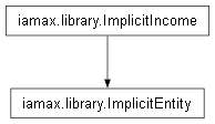

Class that abstracts the idea of economic agents who are just accounting artifacts that need, at some point, to be formalized explicitly.

Note

This class has not vocation to be vectorization friendly since implicit entities are recursively function of each others.

static other_costs_computer(other_costs: np.ndarray)¶

s/e., \(1 \times 1\), denoted as

(167)¶\[v_{\ootau,\ j} = \sum_{k \in \mcI_j} v_{\ootau,\ k}\]

with \(\mcI_j\) the index set required to get \(\mcr_j\).

Parameters: other_costs (numpy.ndarray) – \((\bv_{\ootau,\ k})_{k \in \mcI_j}\), i.e. the \(j\)th \(1 \times |\mcI_j|\) slice of other_costs.

static net_surplus_computer(net_surplus: np.ndarray)¶

s/e., \(1 \times 1\), denoted as

(168)¶\[\pi_{j} = \sum_{k \in \mcI_j} \pi_{k}\]

with \(\mcI_j\) the index set required to get \(\mcr_j\).

Parameters: net_surplus (numpy.ndarray) – \((\bpi_{k})_{k \in \mcI_j}\), i.e. the \(j\)th \(1 \times |\mcI_j|\) slice of net_surplus.

static gross_income_throughput_computer(gross_incomes_throughputs: np.ndarray)¶

s/e., \(1 \times 1\), denoted as

(169)¶\[\mcr_{\text{cum},\ j} = \sum_{k \in \mcI_j} \mcr_{\text{cum},\ k}\]

with \(\mcI_j\) the index set required to get \(\mcr_j\).

Parameters: gross_incomes_throughputs (numpy.ndarray) – \((\bmcr_k)_{\text{cum},\ k \in \mcI_j}\), i.e. the \(j\)th \(1 \times |\mcI_j|\) slice of gross_incomes_throughputs.

static input_values_computer(input_values: np.ndarray)¶

s/e., \(|\mcI_j| \times 1\), denoted as

(170)¶\[\bmcV_{:,j} = \sum_{k \in \mcI_j} \bmcV_{:,k}\]

with \(\mcI_j\) the index set required to get \(\bmcV_{:,j}\).

Parameters: input_values (numpy.ndarray) – \((\bmcV_{:,k})_{k \in \mcI_j}\), i.e. the \(j\)th \(|\mcI| \times |\mcI_j|\) input_values’s slice.

See also

\(\mcI\)’s archetype _iidentifiers.

Example

>>> a = np.hstack((
...     _1s := np.ones((4,))[:, None],
...     _1s.cumsum(axis=0), .5*_1s,
... ))
>>> a
array([[1. , 1. , 0.5],
       [1. , 2. , 0.5],
       [1. , 3. , 0.5],
       [1. , 4. , 0.5]])
>>> ImplicitEntity.input_values_computer(input_values=a)
array([[2.5],
       [3.5],
       [4.5],
       [5.5]])

Let’s vectorize the above example.

>>> (v := np.stack((a, .1*a)))
array([[[1.  , 1.  , 0.5 ],
        [1.  , 2.  , 0.5 ],
        [1.  , 3.  , 0.5 ],
        [1.  , 4.  , 0.5 ]],
       [[0.1 , 0.1 , 0.05],
        [0.1 , 0.2 , 0.05],
        [0.1 , 0.3 , 0.05],
        [0.1 , 0.4 , 0.05]]])
>>> ImplicitEntity.input_values_computer(input_values=v)
array([[[2.5 ],
        [3.5 ],
        [4.5 ],
        [5.5 ]],
       [[0.25],
        [0.35],
        [0.45],
        [0.55]]])

static specific_margins_computer(specific_margins: np.ndarray)¶

s/e., \(|\mcI_j| \times 1\), denoted as

(171)¶\[\bV^{(\utau)}_{:,j} = \sum_{k \in \mcI_j} \bV^{(\utau)}_{:,k}\]

with \(\mcI_j\) the index set required to get \(\bV^{(\utau)}_{:,j}\).

Parameters: specific_margins (numpy.ndarray) – \((\bV^{(\utau)}_{:,k})_{k \in \mcI_j}\), i.e. the \(j\)th \(|\mcI| \times |\mcI_j|\) specific_margins’s slice.

static trade_margins_computer(trade_margins: np.ndarray)¶

s/e., \(|\mcI_j| \times 1\), denoted as

(172)¶\[\bV^{(\jtau)}_{:,j} = \sum_{k \in \mcI_j} \bV^{(\jtau)}_{:,k}\]

with \(\mcI_j\) the index set required to get \(\bV^{(\jtau)}_{:,j}\).

Parameters: trade_margins (numpy.ndarray) – \((\bV^{(\jtau)}_{:,k})_{k \in \mcI_j}\), i.e. the \(j\)th \(|\mcI| \times |\mcI_j|\) trade_margins’s slice.

static sales_taxes_computer(sales_taxes: np.ndarray)¶

s/e., \(|\mcI_j| \times 1\), denoted as

(173)¶\[\bV^{(\htau)}_{:,j} = \sum_{k \in \mcI_j} \bV^{(\htau)}_{:,k}\]

with \(\mcI_j\) the index set required to get \(\bV^{(\htau)}_{:,j}\).

Parameters: sales_taxes (numpy.ndarray) – \((\bV^{(\htau)}_{:,k})_{k \in \mcI_j}\), i.e. the \(j\)th \(|\mcI| \times |\mcI_j|\) sales_taxes’s slice.

static excises_computer(excises: np.ndarray)¶

s/e., \(|\mcI_j| \times 1\), denoted as

(174)¶\[\bV^{(\ctau)}_{:,j} = \sum_{k \in \mcI_j} \bV^{(\ctau)}_{:,k}\]

with \(\mcI_j\) the index set required to get \(\bV^{(\ctau)}_{:,j}\).

Parameters: excises (numpy.ndarray) – \((\bV^{(\ctau)}_{:,k})_{k \in \mcI_j}\), i.e. the \(j\)th \(|\mcI| \times |\mcI_j|\) excises’s slice.

class iamax.library.BalanceOfTrade¶

Accounting entity that consists in a given nation’s net exports.

static budget_constraint_computer(budget_constraints: np.ndarray)¶

s/e., \(1 \times 1\), denoted as

(175)¶\[\mcr_j = \sum_{k=1}^{|\mcI_j|/2} \mcr_k - \sum_{k=1 + |\mcI_j|/2}^{|\mcI_j|} \mcr_k\]

where \(\mcI_j\) is by default asserted to be of even cardinality.

Parameters: budget_constraints (numpy.ndarray) – \((\bmcr_k)_{k \in \mcI_j}\), i.e. the \(j\)th \(1 \times |\mcI_j|\) budget_constraints’s slice.

Important

This method relies on the structure of its argument, with exports concentrated in the first half of budget_constraints and imports in the second.

Example

>>> a = np.array([[4., 16., 3., 2.]])
>>> BalanceOfTrade.budget_constraint_computer(
...     budget_constraints=a
... )
array([[15.]])

Let’s vectorize the above example

>>> (v := np.stack((a, a[:, ::-1])))
array([[[ 4., 16.,  3.,  2.]],
       [[ 2.,  3., 16.,  4.]]])
>>> BalanceOfTrade.budget_constraint_computer(
...     budget_constraints=v
... )
array([[[ 15.]],
       [[-15.]]])

static other_costs_computer(other_costs: np.ndarray)¶

s/e., \(1 \times 1\), denoted as

(176)¶\[v_{\ootau,\ j} = \sum_{k=1}^{|\mcI_j|/2} v_{\ootau,\ k} - \sum_{k=1 + |\mcI_j|/2}^{|\mcI_j|} v_{\ootau,\ k}\]

where \(\mcI_j\) is by default asserted to be of even cardinality.

Parameters: other_costs (numpy.ndarray) – \((\bv_{\ootau,\ k})_{k \in \mcI_j}\), i.e. the \(j\)th \(1 \times |\mcI_j|\) slice of other_costs.

Important

This method relies on the structure of its argument, with exports concentrated in the first half of other_costs and imports in the second.

static net_surplus_computer(net_surplus: np.ndarray)¶

s/e., \(1 \times 1\), denoted as

(177)¶\[\pi_{j} = \sum_{k=1}^{|\mcI_j|/2} \pi_{k} - \sum_{k=1 + |\mcI_j|/2}^{|\mcI_j|} \pi_{k}\]

where \(\mcI_j\) is by default asserted to be of even cardinality.

Parameters: net_surplus (numpy.ndarray) – \((\bpi_{k})_{k \in \mcI_j}\), i.e. the \(j\)th \(1 \times |\mcI_j|\) slice of net_surplus.

Important

This method relies on the structure of its argument, with exports concentrated in the first half of net_surplus and imports in the second.

static gross_income_throughput_computer(gross_incomes_throughputs: np.ndarray)¶

s/e., \(1 \times 1\), denoted as

(178)¶\[\mcr_{\text{cum},\ j} = \sum_{k=1}^{|\mcI_j|/2} \mcr_{\text{cum},\ k} - \sum_{k=1 + |\mcI_j|/2}^{|\mcI_j|} \mcr_{\text{cum},\ k}\]

where \(\mcI_j\) is by default asserted to be of even cardinality.

Parameters: gross_incomes_throughputs (numpy.ndarray) – \((\bmcr_k)_{\text{cum},\ k \in \mcI_j}\), i.e. the \(j\)th \(1 \times |\mcI_j|\) slice of gross_incomes_throughputs.

Important

This method relies on the structure of its argument, with exports concentrated in the first half of gross_incomes_throughputs and imports in the second.

static input_values_computer(input_values: np.ndarray)¶

s/e., \(|\mcI_j| \times 1\), denoted as

(179)¶\[\bmcV_{:,j} = \sum_{k=1}^{|\mcI_j|/2} \bmcV_{:,k} - \sum_{k=1 + |\mcI_j|/2}^{|\mcI_j|} \bmcV_{:,k}\]

with \(\mcI_j\) the index set required to get \(\bmcV_{:,j}\), by default asserted to be of even cardinality.

Parameters: input_values (numpy.ndarray) – \((\bmcV_{:,k})_{k \in \mcI_j}\), i.e. the \(j\)th \(|\mcI| \times |\mcI_j|\) input_values’s slice.

See also

\(\mcI\)’s archetype _iidentifiers.

Example

>>> a = np.hstack((
...     x := np.arange(-2, 3)[:, None],
...     m := np.ones_like(x),
... ))
>>> a
array([[-2,  1],
       [-1,  1],
       [ 0,  1],
       [ 1,  1],
       [ 2,  1]])
>>> BalanceOfTrade.input_values_computer(input_values=a)
array([[-3],
       [-2],
       [-1],
       [ 0],
       [ 1]])

Let’s vectorize the above example.

>>> (v := np.stack((a, -2*a)))
array([[[-2,  1],
        [-1,  1],
        [ 0,  1],
        [ 1,  1],
        [ 2,  1]],
       [[ 4, -2],
        [ 2, -2],
        [ 0, -2],
        [-2, -2],
        [-4, -2]]])
>>> BalanceOfTrade.input_values_computer(input_values=v)
array([[[-3],
        [-2],
        [-1],
        [ 0],
        [ 1]],
       [[ 6],
        [ 4],
        [ 2],
        [ 0],
        [-2]]])

Yet another example with an odd number of trade components.

>>> a = np.hstack((x , np.ones_like(x), m))
>>> (v := np.stack((a, -a)))
array([[[-2,  1,  1],
        [-1,  1,  1],
        [ 0,  1,  1],
        [ 1,  1,  1],
        [ 2,  1,  1]],
       [[ 2, -1, -1],
        [ 1, -1, -1],
        [ 0, -1, -1],
        [-1, -1, -1],
        [-2, -1, -1]]])
>>> BalanceOfTrade.input_values_computer(input_values=v)
array([[[-2],
        [-1],
        [ 0],
        [ 1],
        [ 2]],
       [[ 2],
        [ 1],
        [ 0],
        [-1],
        [-2]]])

static specific_margins_computer(specific_margins: np.ndarray)¶

s/e., \(|\mcI_j| \times 1\), denoted as

(180)¶\[\bV^{(\utau)}_{:,j} = \sum_{k=1}^{|\mcI_j|/2} \bV^{(\utau)}_{:,j} - \sum_{k=1 + |\mcI_j|/2}^{|\mcI_j|} \bV^{(\utau)}_{:,j}\]

with \(\mcI_j\) the index set required to get \(\bV^{(\utau)}_{:,j}\), asserted to be of even cardinality.

Parameters: specific_margins (numpy.ndarray) – \((\bV^{(\utau)}_{:,k})_{k \in \mcI_j}\), i.e. the \(j\)th \(|\mcI| \times |\mcI_j|\) specific_margins’s slice.

static trade_margins_computer(trade_margins: np.ndarray)¶

s/e., \(|\mcI_j| \times 1\), denoted as

(181)¶\[\bV^{(\jtau)}_{:,j} = \sum_{k=1}^{|\mcI_j|/2} \bV^{(\jtau)}_{:,j} - \sum_{k=1 + |\mcI_j|/2}^{|\mcI_j|} \bV^{(\jtau)}_{:,j}\]

with \(\mcI_j\) the index set required to get \(\bV^{(\jtau)}_{:,j}\), asserted to be of even cardinality.

Parameters: trade_margins (numpy.ndarray) – \((\bV^{(\jtau)}_{:,k})_{k \in \mcI_j}\), i.e. the \(j\)th \(|\mcI| \times |\mcI_j|\) trade_margins’s slice.

static sales_taxes_computer(sales_taxes: np.ndarray)¶

s/e., \(|\mcI_j| \times 1\), denoted as

(182)¶\[\bV^{(\htau)}_{:,j} = \sum_{k=1}^{|\mcI_j|/2} \bV^{(\htau)}_{:,j} - \sum_{k=1 + |\mcI_j|/2}^{|\mcI_j|} \bV^{(\htau)}_{:,j}\]

with \(\mcI_j\) the index set required to get \(\bV^{(\htau)}_{:,j}\), asserted to be of even cardinality.

Parameters: sales_taxes (numpy.ndarray) – \((\bV^{(\htau)}_{:,k})_{k \in \mcI_j}\), i.e. the \(j\)th \(|\mcI| \times |\mcI_j|\) sales_taxes’s slice.

static excises_computer(excises: np.ndarray)¶

s/e., \(|\mcI_j| \times 1\), denoted as

(183)¶\[\bV^{(\ctau)}_{:,j} = \sum_{k=1}^{|\mcI_j|/2} \bV^{(\ctau)}_{:,j} - \sum_{k=1 + |\mcI_j|/2}^{|\mcI_j|} \bV^{(\ctau)}_{:,j}\]

with \(\mcI_j\) the index set required to get \(\bV^{(\ctau)}_{:,j}\), asserted to be of even cardinality.

Parameters: excises (numpy.ndarray) – \((\bV^{(\ctau)}_{:,k})_{k \in \mcI_j}\), i.e. the \(j\)th \(|\mcI| \times |\mcI_j|\) excises’s slice.

class iamax.library.AQConserver¶

Class that captures the essence of the conservation law regarding additive quantities.

static additive_output_volume_rooter(output_volume: np.ndarray, aggregated_input_volumes: np.ndarray)¶

s/e., \(1 \times 1\) unit-dimensionless zero.

(184)¶\[\approx 0\]

Parameters

output_volume (float) – \(q_j\), i.e. the \(j\)th \(1 \times 1\) output_volumes’s element.
aggregated_input_volumes (numpy.ndarray) – \((\bq^{T,\text{drate}}_{k,1})_{k \in \mcI_j}\), i.e. the \(j\)th \(1 \times |\mcI_j|\) aggregated_input_volumes’s slice.

Example

>>> ovol   = 10.
>>> aivols = np.array([[6., 4.]])
>>> AQConserver.additive_output_volume_rooter(
...     output_volume=ovol, aggregated_input_volumes=aivols,
... )
array([[0.]])

>>> vovol = np.array([[[ovol]], [[.5*ovol]]])
>>> vovol
array([[[10.]],
       [[ 5.]]])
>>> vaivols = np.stack((aivols, .5*aivols[..., ::-1]))
>>> vaivols
array([[[6., 4.]],
       [[2., 3.]]])
>>> AQConserver.additive_output_volume_rooter(
...     output_volume=vovol, aggregated_input_volumes=vaivols,
... )
array([[[0.]],
       [[0.]]])

class iamax.library.SymmetricNodes¶

Class that captures the essence of entities balancing each other out through gross_income_throughput attribute.

static gross_income_throughput_rooter(gross_incomes_throughputs: np.ndarray)¶

s/e., \(1 \times 1\) unit-dimensionless zero.

Parameters

gross_incomes_throughputs (numpy.ndarray) – \((\bmcr_k)_{\text{cum},\ k \in \mcI_j}\), i.e. the \(j\)th \(1 \times |\mcI_j|\) slice of gross_incomes_throughputs.

Example

>>> a = np.array([[.9, -.9]])
>>> SymmetricNodes.gross_income_throughput_rooter(
...     gross_incomes_throughputs=a
... )
array([[0.]])

Let’s vectorize the above example.

>>> v = np.stack((
...     np.array([[.5, -.5]]),
...     np.array([[.0, -.5]]),
...     np.array([[.5,  .0]]),
... ))
>>> SymmetricNodes.gross_income_throughput_rooter(
...     gross_incomes_throughputs=v
... )
array([[[ 0.]],
       [[ 1.]],
       [[-1.]]])

class iamax.library.BalancedWorldTrade¶

Class that refers to the requirement in international economics that the sum of all trade balances across regions must equal zero. This identity reflects the idea that every export is matched by an import somewhere else, ensuring that total exports equal total imports when viewed globally.

Note

This class assumes that world trade is resolved in terms of physical volumes.

static spendings_dfree_rooter(spendings_dfree: np.ndarray)¶

s/e., \(1 \times 1\) unit-dimensionless zero.

Parameters

spendings_dfree (numpy.ndarray) – \((\bmcv_k)_{\neg\ttau,\ k \in \mcI_j}\), i.e. the \(j\)th \(1 \times |\mcI_j|\) slice of spendings_dfree.

Example

>>> a = np.array([[.9, -.9]])
>>> BalancedWorldTrade.spendings_dfree_rooter(
...     spendings_dfree=a
... )
array([[0.]])

Let’s vectorize the above example.

>>> v = np.stack((
...     np.array([[.5, -.5]]),
...     np.array([[.0, -.5]]),
...     np.array([[.5,  .0]]),
... ))
>>> BalancedWorldTrade.spendings_dfree_rooter(
...     spendings_dfree=v
... )
array([[[ 0.]],
       [[ 1.]],
       [[-1.]]])

class iamax.library.Shareholders¶

Class that abstracts the idea of agents who jointly own 100% of an activity’s outstanding shares.

static income_private_circuit_rsto_rooter(income_private_circuit_rsto: np.ndarray)¶

s/e., \(1 \times 1\) unit-dimensionless zero.

(185)¶\[\approx 0\]

Parameters: income_private_circuit_rsto (numpy.ndarray) – \((\obtheta_{k})_{k \in \mcI_j}\), i.e. a \(1 \times |\mcI_j|\) slice of income_private_circuit_rsto.

See also

income_private_circuit_rsto.

Example

>>> a = np.array([[.9]])
>>> Shareholders.income_private_circuit_rsto_rooter(
...     income_private_circuit_rsto=a
... )
array([[-0.1]])

Let’s vectorize the above example.

>>> (v := np.stack((a, 1 - a, a + .1)))
array([[[0.9]],
       [[0.1]],
       [[1. ]]])
>>> Shareholders.income_private_circuit_rsto_rooter(
...     income_private_circuit_rsto=v
... )
array([[[-0.1]],
       [[-0.9]],
       [[ 0. ]]])

class iamax.library.Accountant¶

Static class (to be inherited) that aggregates a bunch of methods related to accounting equations.

static output_price_computer(*, output_volume: float, input_values: np.ndarray)¶

s/e., \(1 \times 1\).

(186)¶\[\up_j = \frac{\sum_{k \in \mcI_j} \mcv_k}{q_j}\]

with \(\mcI_j\) the index set required to get \(\up_j\).

Parameters

output_volume (float) – \(q_j\), i.e. the \(j\)th \(1 \times 1\) output_volumes’s element.
input_values (numpy.ndarray) – \((\bmcV_{k,j})_{k \in \mcI_j}\), i.e. the \(j\)th \(1 \times |\mcI_j|\) input_values’s slice.

See also

output_prices.

Example

>>> a = 1.
>>> b = np.array([[1., 9.]])
>>> Accountant.output_price_computer(
...     output_volume=a, input_values=b
... )
array([[10.]])

Let’s vectorize the above example

>>> Accountant.output_price_computer(
...     output_volume=np.atleast_2d([a, 5*a]).T,
...     input_values=np.vstack((b, b))
... )
array([[10.],
       [ 2.]])

class iamax.library.CoInitiatedVolumes(scaling_factor: float = 1.0)¶

Class that abstracts the concept of (independent) volumes whose initial state are yet to be determined jointly.

Parameters: scaling_factor (float) – S/e. set to 1 by default.

output_volumes_ccomputer(self, *, input_values: np.ndarray, additive_output_volumes: np.ndarray)¶

s/e.

Parameters

additive_output_volumes (numpy.ndarray) – \(q_j\), i.e. the \(j\)ths \(1 \times 1\) additive_output_volumes’s elements, whose last component only is of interest.
input_values (numpy.ndarray) – \((\bmcV_{kk,j})_{k \in \mcI_j}\), i.e. the \(j\)th \(|\mcI_j| \times |\mcI_j| + 1\) input_values’s slice (diagonal) rectangular slice.

Important

This method relies on the structure of its argument, as outlined in the description of argument additive_output_volumes.

Attention

By appending its output with a 0, this method overwrites the last component of the targeted attribute.

class iamax.library.BalancedSM¶

Class that abstracts the concept of specific margins summing to zero across consumers subjected to it.

static specific_margin_balance_rooter(specific_margins_balances: np.ndarray)¶

s/e., \(1 \times 1\) unit-dimensionless zero.

Parameters

specific_margins_balances (numpy.ndarray) – \(\bv_{\utau,\ j}\), i.e. the \(j\)th \(1 \times 1\) element of specific_margins_balances.

Example

>>> a = np.array([[.9]])
>>> BalancedSM.specific_margin_balance_rooter(
...     specific_margins_balances=a
... )
array([[0.9]])

Let’s vectorize the above example.

>>> v = np.stack((
...     np.array([[.5]]),
...     np.array([[.0]]),
...     np.array([[.5]]),
... ))
>>> BalancedSM.specific_margin_balance_rooter(
...     specific_margins_balances=v
... )
array([[[0.5]],
       [[0. ]],
       [[0.5]]])

class iamax.library.InitiallyBalancedSM¶

BalancedSM’s counterpart that restricts the balancing at time t=0.

static specific_margin_balance_crooter(specific_margins_balances: np.ndarray)¶

s/e., \(1 \times 1\) unit-dimensionless zero.

Parameters

specific_margins_balances (numpy.ndarray) – \(\bv_{\utau,\ j}\), i.e. the \(j\)th \(1 \times 1\) specific_margins_balances’s element.

Example

>>> a = np.array([[.9]])
>>> InitiallyBalancedSM.specific_margin_balance_crooter(
...     specific_margins_balances=a
... )
array([[0.9]])

Let’s vectorize the above example.

>>> v = np.stack((
...     np.array([[.5]]),
...     np.array([[.0]]),
...     np.array([[.5]]),
... ))
>>> InitiallyBalancedSM.specific_margin_balance_crooter(
...     specific_margins_balances=v
... )
array([[[0.5]],
       [[0. ]],
       [[0.5]]])

Constant Elasticity of Substitution base class and/or mixin class.

Parameters

sigma (float or np.ndarray) – The elasticity of substitution \(\sigma\), with the substitution parameter being defined as \(\rho = \frac{\sigma - 1}{\sigma}\).
nu (float) – The degree of homogeneity of the aggregation \(\nu\), set to 1. by default.
eta (float) – The responsiveness parameter \(\eta\), used under dynamic circumstances, if any. Set to .0 by default.

Note

This class can either be linear, Cobb–Douglas or Leontief:

If \((\sigma \to \infty) \iff (\rho \to 1)\), we get a linear or perfect substitutes function;

If \((\sigma \to 1) \iff (\rho \to 0)\), we get a Cobb–Douglas function;

If \((\sigma \to 0) \iff (\rho \to -\infty)\), we get a Leontief or perfect complements function.

Example

>>> CES(sigma=0).aggregation_type
'Leontief'
>>> CES(sigma=.5).aggregation_type
'Gross complements'
>>> CES(sigma=1).aggregation_type
'Cobb–Douglas'
>>> CES(sigma=2).aggregation_type
'Imperfect Substitutes'
>>> CES(sigma=np.inf).aggregation_type
'Perfect substitutes'
>>> CES(sigma=[0, 1, np.inf]).aggregation_type
['Leontief', 'Cobb–Douglas', 'Perfect substitutes']

property aggregation_type(self)¶

Aggregation qualifier, be this aggregation related to cardinal (e.g. production) or ordinal (e.g. utility level) quantities.

Example

>>> CES(sigma=[0, 1, np.inf]).aggregation_type
['Leontief', 'Cobb–Douglas', 'Perfect substitutes']

property sigma(self)¶: Elasticity of substitution \(\sigma\).

property rho(self)¶: Substitution parameter \(\rho\).

property nu(self)¶: Aggregation’s degree of homogeneity \(\nu\).

property eta(self)¶: Responsiveness to input price changes \(\eta\).

abstract compute_calibrand_0(self, **kwargs: float)¶: Method to be called during calibration.

Attention

This method is assumed (but not asserted) to only be dealing with Keyword-Only Arguments.

Warning

This method will likely be reattached as soon as a technology (or preference) morphism being ontologically upstream of CES is defined.

static _aggregator(*, shares: np.ndarray, aggregands: np.ndarray, rho: float, nu_rho_inv: float)¶

Class’s core morphism, \(1 \times 1\), denoted as

(187)¶\[y = \left( \sum_{i=1}^n a_{i} x_{i}^{\rho} \right)^\frac{\nu}{\rho}\]

where \(y\) is the quantity of aggregate, \(x_i\) the quantity of \(i\)-aggregand, \(a_i\) its associated share, \(\rho\) the substitution parameter and \(\nu\) the degree of homogeneity of the aggregation.

Note

This method is vectorization friendly over the 0th axis. Incidentally, it may also be turned into instance method once the developments stabilize.

Parameters

shares (numpy.ndarray) – \(1 \times n\) archetype of the distribution parameters.
aggregands (numpy.ndarray) – \(1 \times n\) archetype of the aggregands.
rho (float) – \(1 \times 1\) archetype of the substitution parameter.
nu_rho_inv (float) – Precomputed \(1 \times 1\) archetype of aggregation degree of homogeneity multiplied by the inverse of the substitution parameter.

Example

>>> a = np.array([[0.29151, 0.95657]])
>>> b = np.array([[1782.232, 19190.896]])
>>> CES._aggregator(
...     shares=a, aggregands=b,
...     rho=.5, nu_rho_inv=2.
... )
array([[20973.22]])

Let’s vectorize the above example

>>> CES._aggregator(
...     shares=np.vstack((a, a)),
...     aggregands=np.vstack((b, b)),
...     rho=np.atleast_2d([.5, .0]).T,
...     nu_rho_inv=2.
... )
array([[2.10e+04],
       [1.56e+00]])

class iamax.library.HicksianCES(*args, **kwargs)¶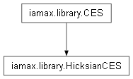

Inheritance diagram of iamax.library.HicksianCES

Constant Elasticity of Substitution abstraction whose optimal demand function derives from a maximization program formulated à la Hicks.

Note

Calculations assert constant return to scale, i.e. Eq.187’s \(\nu\) is forced to be \(1\) at instantiation.

compute_calibrand_0(self, *, output_volume: float|np.ndarray, input_volumes: np.ndarray, input_values: np.ndarray)¶

This method supports the FOC-based calibration of \((a_{k,j})_{k \in \mcI_j}\), the \(|\mcI_j|\) demand distribution parameters related to aggregate \(j\),

(188)¶\[a_k = \left[ \left( \frac{\mcv_k}{\sum_{k' \in \mcI_j} \mcv_{k'}} \right)^{ \text{I}(\rho_j \neq -\infty) } \left(\frac{q_j}{q_k}\right)^{ \rho_j^{\text{I}(\rho_j \neq -\infty)} } \right]^{\text{I}(\rho_j \neq 1)}, \ \forall k \ \in \mcI_j\]

with \(q_j\) the output level to be satisfied, \(\rho_j\) the substitution parameter, \(\mcI_j\) the index set of inputs required by \(q_j\)’s underlying technology, \(q_k\) the optimal level of input required to meet \(q_j\), \(\mcv_k\) the \(q_k\)’s input value and \(\text{I}(\cdot)\) an indicator function returning the trueness of the statement being passed as argument.

Parameters

output_volume (float) – \(q_j\), i.e. the \(j\)th \(1 \times 1\) output_volumes’s element.
input_volumes (numpy.ndarray) – \((\bQ_{k,j})_{k \in \mcI_j}\), i.e. the \(j\)th \(1 \times |\mcI_j|\) input_volumes’s slice.
input_values (numpy.ndarray) – \((\bmcV_{k,j})_{k \in \mcI_j}\), i.e. the \(j\)th \(1 \times |\mcI_j|\) input_values’s slice.

Example

>>> ovol  = 20973.128
>>> ivols = np.array([[1782.232, 19190.896]])
>>> ivals = 1e3*ivols

>>> h = HicksianCES(sigma=2.)
>>> _ = h.compute_calibrand_0(
...     output_volume = ovol,
...     input_volumes = ivols,
...     input_values  = ivals,
... )
>>> h.calibrand_0
array([[0.29, 0.96]])

Let’s illustrate how such calculation can be vectorized along the 0th axis.

>>> vovol  = np.array([[[ovol]], [[ovol]]])
>>> vivols = np.stack((ivols, .1*ivols))
>>> vivals = 1e3*vivols

>>> h.compute_calibrand_0(
...     output_volume = vovol,
...     input_volumes = vivols,
...     input_values  = vivals,
... ).calibrand_0
array([[[0.29, 0.96]],
       [[0.92, 3.02]]])

The non-constant instantiation parameters case follows.

>>> h = HicksianCES(sigma=[[[2.]], [[3.]]])
>>> _ = h.compute_calibrand_0(
...     output_volume = vovol,
...     input_volumes = vivols,
...     input_values  = vivals,
... )
>>> h.calibrand_0
array([[[0.29, 0.96]],
       [[2.04, 4.51]]])

See also

compute_calibrand_0().

compute_calibrand_0_star(self, *, ioq_shares_drates: np.ndarray, ioq_shares_drates2: np.ndarray, ioq_productivities_drates: np.ndarray, ioq_productivities_drates2: np.ndarray)¶

Define calibrand_0_star, i.e. a version of calibrand_0 that internalizes (crises-like) shocks,

(189)¶\[\begin{split}a_k^{*} &= a_k \left( 1 + \beta^{\text{drate}}_k + \beta^{\text{drate}^{ii}}_k \right)^{ \rho_j^{\text{I}(\rho_j \neq -\infty)} \text{I}(\rho_j \neq 1) } \\ & \left( 1 + \alpha^{-1,\ \text{drate}}_k + \alpha^{-1,\ \text{drate}^{ii}}_k \right)^{\text{I}(\rho_j = -\infty)}, \ \forall k \ \in \mcI_j\end{split}\]

where \(a_k\) and \(\rho_j\) are as defined in Eq.188, \(\beta^\text{drate}_k\) and \(\beta^{\text{drate}^{ii}}_k\) are respectively a crisis-like shock and a spread from it, \(\alpha^{-1,\ \text{drate}^{ii}}_k\) and \(\alpha^{-1,\ \text{drate}}_k\) are, respectively, a scenarized productivity (discrete) growth and a spread from it.

Parameters

ioq_shares_drates (numpy.ndarray) – \((\bbeta^\text{drate}_{k,j})_{k \in \mcI_j}\), i.e. the \(j\)th \(1 \times |\mcI_j|\) ioq_shares_drates’s slice.
ioq_shares_drates2 (numpy.ndarray) – \((\bbeta^{\text{drate}^{ii}}_{k,j})_{k \in \mcI_j}\), i.e. the \(j\)th \(1 \times |\mcI_j|\) ioq_shares_drates2’s slice.
ioq_productivities_drates (numpy.ndarray) – \((\balpha^{-1,\ \text{drate}_{k,j}})_{k \in \mcI_j}\), i.e. the \(j\)th \(1 \times |\mcI_j|\) ioq_productivities_drates’s slice.
ioq_productivities_drates2 (numpy.ndarray) – \((\balpha^{-1,\ \text{drate}^{ii}_{k,j}})_{k \in \mcI_j}\), i.e. the \(j\)th \(1 \times |\mcI_j|\) ioq_productivities_drates2’s slice.

Note

ioq_productivities_drates has vocation to “overwrite” ioq_shares_drates sooner or later.

Important

Keep in mind that \(a_k\) and \(\rho_j\) are internally handled as instance attributes, i.e. in the same manner as calibrand_0 and rho.

allege_input_shares(self, *, input_prices: np.ndarray, input_prices_lagged: np.ndarray, ioq_intensities_lagged: np.ndarray)¶

Alleged input shares, \(1 \times |\mcI_j|\), denoted as

(190)¶\[s_{k,t} = \frac{ s_{k,t-1} \left( p_{k,t} / p_{k,t-1} \right)^{\eta_j} }{ \sum_{k^{'} \in \mcI_j} s_{k^{'},t-1} \left( p_{k^{'},t} / p_{k^{'},t-1} \right)^{\eta_j} } \ \forall k \ \in \mcI_j\]

where \(\eta_j\) is a \(j\)-specific responsiveness parameter and \(\mcI_j\) and \(p_k\) are as described in Eq.194.

Parameters

input_prices (numpy.ndarray) – \((\tbP_{k,j})_{k \in \mcI_j}\), i.e. the \(j\)th \(1 \times |\mcI_j|\) input_prices’s slice.
input_prices_lagged (numpy.ndarray) – \((\tbP_{k,j})_{k \in \mcI_j}\), i.e. the \(j\)th \(1 \times |\mcI_j|\) slice of the lagged version of input_prices.
ioq_intensities_lagged (numpy.ndarray) – \((\balpha_{k,j})_{k \in \mcI_j}\), i.e. the \(j\)th \(1 \times |\mcI_j|\) slice of the lagged version of ioq_intensities.

Example

>>> invariants = dict(
...     input_prices           = np.array([[1., 1.25]]),
...     input_prices_lagged    = np.array([[1., 1.]]),
...     ioq_intensities_lagged = np.array([[.4, .6]]),
... )

>>> HicksianCES(
...     sigma=np.inf, eta=0.
... ).allege_input_shares(**invariants).alleged_input_shares
array([[0.4, 0.6]])
>>> HicksianCES(
...     sigma=np.inf, eta=1.
... ).allege_input_shares(**invariants).alleged_input_shares
array([[0.35, 0.65]])
>>> HicksianCES(
...     sigma=np.inf, eta=4.
... ).allege_input_shares(**invariants).alleged_input_shares
array([[0.21, 0.79]])

compute_input_volumes_shocks(self, *, input_volumes_drates: np.ndarray)¶

s/e., \(1 \times |\mcI_j|\), calculated and assigned to attribute input_volumes_shocks since required in several methods of the instance.

(191)¶\[\bQ^\text{dmult}_j = 1 + \bQ^\text{drate}_j\]

Parameters: input_volumes_drates (numpy.ndarray) – \((\bQ^\text{drate}_{k,j})_{k \in \mcI_j}\), i.e. the \(j\)th \(1 \times |\mcI_j|\) input_volumes_drates’s slice.

Note

Since the name of this method mirrors nothing within the list of eligible variables (be them related to targets or arguments), it will be assumed to work in place.

Important

Keep in mind that input_volumes_shocks is defined and internally handled as instance attributes, cf. the example section below.

Example

>>> h = HicksianCES(sigma=None)
>>> h.compute_input_volumes_shocks(
...     input_volumes_drates=np.array([[.1, .2]])
... ).input_volumes_shocks
array([[1.1, 1.2]])

_output_volume_computer(self, *, input_volumes: np.ndarray)¶

Output supply, \(1 \times 1\), denoted as

(192)¶\[q_j = \left( \sum_{k \in \mcI_j} a_k q_k^{ \rho_j^{ \text{I}(\rho_j\neq-\infty) } } \right)^{ \rho_j^{ -\text{I}(\rho_j\neq-\infty) } } |\mcI_j|^{ -\text{I}(\rho_j=-\infty) }\]

where \(\mcI_j\), \(q_j\), \(q_k\), \(a_k\), \(\rho_j\) and \(\text{I}(\cdot)\) are as described in Eq.188.

Note

Eq.192 is unconditionally valid only when \(q_{k=1, \ldots, |\mcI_j|}\)’s levels are the optimal input demands’.

Parameters

input_volumes (numpy.ndarray) – \((\bQ_{k,j})_{k \in \mcI_j}\), i.e. the \(j\)th \(1 \times |\mcI_j|\) input_volumes’s slice.

Example

>>> ovol  = 20973.128
>>> ivols = np.array([[1782.232, 19190.896]])
>>> ivals = 1e3*ivols

>>> h = HicksianCES(sigma=2.)
>>> _ = h.compute_calibrand_0(
...     output_volume = ovol,
...     input_volumes = ivols,
...     input_values  = ivals
... )
>>> h._output_volume_computer(
...     input_volumes = ivols,
... )
array([[20973.13]])

Let’s illustrate how such calculation can be vectorized along the 0th axis.

>>> vovol  = np.array([[[ovol]], [[.5*ovol]], [[ovol]]])
>>> vivols = np.stack((ivols, .5*ivols, ivols))
>>> vivals = 1e3*vivols

>>> _ = h.compute_calibrand_0(
...     output_volume = vovol,
...     input_volumes = vivols,
...     input_values  = vivals,
... )
>>> h._output_volume_computer(
...     input_volumes = vivols,
... )
array([[[20973.13]],
       [[10486.56]],
       [[20973.13]]])

compute_output_price_driver(self, *, output_price_drate: np.ndarray)¶: s/e.

output_price_computer(self, *, input_prices: np.ndarray)¶

s/e., \(1 \times 1\).

(193)¶\[\up_j = \left( \sum_{k \in \mcI_j} \left[ a_k^{ (-1)^{\text{I}(\sigma_j = 0)} \sigma_j^{\text{I}(\sigma_j \neq 0)} } \right]^{\text{I}(\sigma_j \neq \infty)} p_k^{ (1 - \sigma_j)^{\text{I}(\sigma_j \neq \infty)} } s_k^{\text{I}(\sigma_j = \infty)} \right)^{ (1 - \sigma_j)^{-\text{I}(\sigma_j \neq \infty)} }\]

where \(\mcI_j\), \(a_k\) and \(\text{I}(\cdot)\) are as in Eq.188, \(\sigma_j\) and \(p_k\) are as in Eq.194, \(\up_j\) is the output’s producer price and \(s_k\) is as in Eq.190.

Parameters: input_prices (numpy.ndarray) – \((\tbP_{k,j})_{k \in \mcI_j}\), i.e. the \(j\)th \(1 \times |\mcI_j|\) input_prices’s slice.

See also

output_prices.

Important

This method overrides its (parent) output_price_computer counterpart.

Example

>>> ovol  = 20973.128
>>> ivols = np.array([[1782.232, 19190.896]])
>>> iprcs = np.array([[1000., 1000.]])
>>> ivals = iprcs*ivols

>>> h = HicksianCES(sigma=2.)
>>> _ = h.compute_calibrand_0(
...     output_volume = ovol,
...     input_volumes = ivols,
...     input_values  = ivals,
... )
>>> h.output_price_computer(
...     input_prices = iprcs,
... ).item()
1000.0

Let’s illustrate how such calculation can be vectorized over the 0th axis.

>>> vovol  = np.array([[[ovol]], [[.5*ovol]], [[ovol]]])
>>> vivols = np.stack((ivols, .5*ivols, ivols))
>>> vivals = 1e3*vivols
>>> viprcs = 1e3*np.ones_like(vivols)

>>> _ = h.compute_calibrand_0(
...     output_volume = vovol,
...     input_volumes = vivols,
...     input_values  = vivals,
... )
>>> h.output_price_computer(
...     input_prices = viprcs,
... )
array([[[1000.]],
       [[1000.]],
       [[1000.]]])

input_volumes_computer(self, *, output_volume: float|np.ndarray, input_prices: np.ndarray)¶

Input demands, \(1 \times |\mcI_j|\), denoted as

(194)¶\[\begin{split}q_k &= q_j \left[ \alpha_k \left(\frac{\up_j}{p_k}\right)^{\sigma_j} \right]^{\text{I}(\sigma_j \neq \infty)} \left[s_k\right]^{\text{I}(\sigma_j = \infty)} \\ &= q_j \left[ \alpha_k p_k^{-\sigma_j} \left( \sum_{k' \in \mcI_j} \alpha_{k'} p_{k'}^{1 - \sigma_j} \right)^{ \frac{\sigma_j}{1 - \sigma_j} } \right]^{\text{I}(\sigma_j \neq \infty)} \left[s_k\right]^{\text{I}(\sigma_j = \infty)}, \ \forall k \ \in \mcI_j\end{split}\]

where \(\alpha_k=a_k^{(-1)^{\text{I}(\sigma_j = 0)} \sigma_j^{\text{I}(\sigma_j \neq 0)}}\) and \(\mcI_j\), \(q_j\), \(q_k\), \(a_k\) and \(\text{I}(\cdot)\) are as in Eq.188, \(p_k\) is the \(q_k\)’s price and \(s_k\) is as described in Eq.190.

Parameters

output_volume (float) – \(q_j\), i.e. the \(j\)th \(1 \times 1\) output_volumes’s element.
input_prices (numpy.ndarray) – \((\tbP_{k,j})_{k \in \mcI_j}\), i.e. the \(j\)th \(1 \times |\mcI_j|\) input_prices’s slice.

Example

>>> ovol  = 20973.128
>>> ivols = np.array([[1782.232, 19190.896]])
>>> iprcs = np.array([[1000., 1000.]])
>>> ivals = iprcs*ivols

>>> h = HicksianCES(sigma=2)
>>> _ = h.compute_calibrand_0(
...     output_volume = ovol,
...     input_volumes = ivols,
...     input_values  = ivals,
... )
>>> h.input_volumes_computer(
...     output_volume = ovol,
...     input_prices  = iprcs,
... )
array([[ 1782.23, 19190.9 ]])

Let’s illustrate how such calculation can be vectorized over the 0th axis.

>>> h      = HicksianCES(sigma=[[[2.]], [[2.]], [[.5]]])
>>> vovol  = np.array([[[ovol]], [[ovol]], [[ovol]]])
>>> vivols = np.stack((ivols, ivols[:, ::-1], ivols))
>>> vivals = 1e3*vivols
>>> viprcs = 1e3*np.ones((3, 1, 2))

>>> h.compute_calibrand_0(
...     output_volume = vovol,
...     input_volumes = vivols,
...     input_values  = vivals,
... ).input_volumes_computer(
...     output_volume = vovol,
...     input_prices  = viprcs,
... )
array([[[ 1782.23, 19190.9 ]],
       [[19190.9 ,  1782.23]],
       [[ 1782.23, 19190.9 ]]])

Once again, but moving away from the calibration context regarding relative prices.

>>> viprcs[..., 0] *= .5
>>> h.input_volumes_computer(
...     output_volume = vovol,
...     input_prices  = viprcs,
... )
array([[[ 6055.96, 16302.5 ]],
       [[20931.83,   485.98]],
       [[ 2457.72, 18713.25]]])

class iamax.library.HicksianICES(*args, **kwargs)¶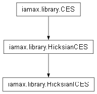

Inheritance diagram of iamax.library.HicksianICES

Ordinal-production altered version of HicksianCES.

Important

At the moment, this method cannot be instantiated at \(\sigma \to \infty\) since it would require MSystem to be endowed with a new economic attribute k.a. iwq_intensities.

compute_calibrand_0(self, *, ordinal_volume: float|np.ndarray, input_volumes: np.ndarray, input_values: np.ndarray)¶: s/e.

See also

compute_calibrand_0.

abstract static allege_input_shares()¶

LSP-offending (in-place) computer.

See also

The reason why this method is nullified.

Example

>>> HicksianICES.allege_input_shares()
Traceback (most recent call last):
 ...
NotImplementedError: Require `core.MSystem.iwq_intensities`

ordinal_volume_computer(self, *, input_volumes: np.ndarray)¶: s/e.

See also

_output_volume_computer.

static compute_output_price_driver()¶: LSP-offending (in-place) computer.

static output_price_computer()¶: LSP-offending (in-place) computer.

input_volumes_computer(self, *, ordinal_volume: float|np.ndarray, input_prices: np.ndarray)¶: s/e.

class iamax.library.HicksianPICES(*args, scaling_factor: float = 1.0, **kwargs)¶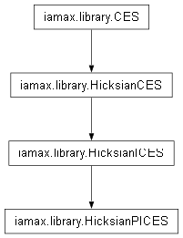

Inheritance diagram of iamax.library.HicksianPICES

Augmented version of HicksianICES that also computes the price of the ordinal quantities being generated.

Parameters: scaling_factor (float) – Ordinal price scaling factor. To 1 by default.

compute_ordinal_price_driver(self, *, ordinal_price_drate: np.ndarray)¶: s/e.

ordinal_price_computer(self, *, input_prices: np.ndarray)¶: s/e.

class iamax.library.ScHicksianCES¶

Inheritance diagram of iamax.library.ScHicksianCES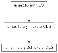

HicksianCES’s altered version whose calibrands determination is solver based.

compute_calibrand_0(self, *, ioq_intensities_drates: np.ndarray)¶: s/e.

ioq_intensities_drates_crooter(self, *, input_volumes: np.ndarray, input_prices: np.ndarray)¶: s/e.

class iamax.library.SmHicksianCES¶

Inheritance diagram of iamax.library.SmHicksianCES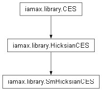

HicksianCES’s altered version whose calibrands determination is softmax-based.

compute_calibrand_0(self, *, input_prices: np.ndarray, input_volumes: np.ndarray)¶

This method supports the softmax-derived calibration of \((a_{k,j})_{k \in \mcI_j}\), the \(|\mcI_j|\) demand distribution parameters related to aggregate \(j\),

(195)¶\[a_k = \left[ \frac{ p_{k}q_{k}^{1/\sigma_j} }{ \sum_{k' \in \mcI_j} p_{k'}q_{k'}^{1/\sigma_j} } \right]^{\text{I}(\sigma_j \neq \infty)}, \ \forall k \ \in \mcI_j\]

with \(\sigma_j\) the elasticity of substitution, \(\mcI_j\) the index set of inputs required by \(q_j\)’s underlying technology, \(q_k\) the optimal level of input required to meet \(q_j\), \(p_k\) the \(q_k\)’s associated input price and \(\text{I}(\cdot)\) an indicator function returning the trueness of the statement being passed as argument.

Parameters

input_prices (numpy.ndarray) – \((\tbP_{k,j})_{k \in \mcI_j}\), i.e. the \(j\)th \(1 \times |\mcI_j|\) input_prices’s slice.
input_volumes (numpy.ndarray) – \((\bQ_{k,j})_{k \in \mcI_j}\), i.e. the \(j\)th \(1 \times |\mcI_j|\) input_volumes’s slice.

class iamax.library.HicksianFCES¶

Inheritance diagram of iamax.library.HicksianFCES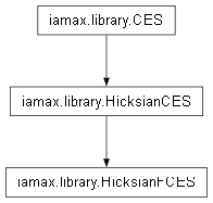

HicksianCES’s altered version whose underlying trade-off is forced.

static allege_input_shares()¶: LSP-offending (in-place) computer.

static compute_input_volumes_shocks()¶: LSP-offending computer.

static input_volumes_computer()¶: LSP-offending computer.

aggregated_input_volumes_rooter(self, *, output_volume: np.ndarray, input_volumes: np.ndarray)¶

s/e., \(1 \times 1\) unit-dimensionless zero.

(196)¶\[\approx 0\]

Parameters

output_volume (float) – \(q_j\), i.e. the \(j\)th \(1 \times 1\) output_volumes’s element.
input_volumes (numpy.ndarray) – \((\bQ_{k,j})_{k \in \mcI_j}\), i.e. the \(j\)th \(1 \times |\mcI_j|\) input_volumes’s slice.

See also

aggregated_input_volumes.

class iamax.library.HicksianACES¶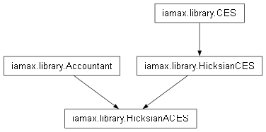: HicksianCES’s altered version whose costs calculation is based on accounting rules.

class iamax.library.HicksianAFCES¶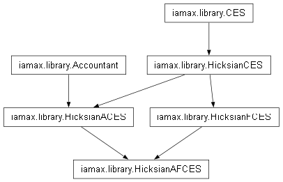: HicksianACES’s altered version whose underlying trade-off is forced.

class iamax.library.HicksianGAFCES(*args, negated_mask: bool = False, **kwargs)¶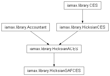

Inheritance diagram of iamax.library.HicksianGAFCES

HicksianACES’s altered version whose underlying trade-off is forced in a generalized manner by restricting it to a consumption subset of arbitrary size.

Parameters: negated_mask (bool) – Whether the mask passed as argument input_volumes_drates2 of the method compute_calibrand_0 is to be negated. Argument input_volumes_drates2 indeed boolean-specifies the goods being freely subject to trade-off by default. Set to False by default.

Attention

This class isn’t well tested for sigma!=0 cases yet, which condition is not asserted (!)

compute_calibrand_0(self, *, output_volume: float|np.ndarray, input_values: np.ndarray, input_volumes: np.ndarray, input_volumes_drates2: np.ndarray)¶

Altered version of compute_calibrand_0.

Parameters

output_volume (float) – \(q_j\), i.e. the \(j\)th \(1 \times 1\) output_volumes’s element.
input_volumes (numpy.ndarray) – \((\bQ_{k,j})_{k \in \mcI_j}\), i.e. the \(j\)th \(1 \times |\mcI_j|\) input_volumes’s slice.
input_values (numpy.ndarray) – \((\bmcV_{k,j})_{k \in \mcI_j}\), i.e. the \(j\)th \(1 \times |\mcI_j|\) input_values’s slice.
input_volumes_drates2 (numpy.ndarray) – \((\bQ^\text{drate}_{k,j})_{k \in \mcI_j}\), i.e. the \(j\)th \(1 \times |\mcI_j|\) input_volumes_drates2’s slice.

Example

>>> ovol  = 20973.128
>>> ivols = np.array([[1782.232, 19190.896]])
>>> ivals = 1e3*ivols
>>> imsks = np.array([[1, 0]])

>>> h = HicksianGAFCES(sigma=0, negated_mask=False)
>>> _ = h.compute_calibrand_0(
...     output_volume         = ovol,
...     input_volumes         = ivols,
...     input_values          = ivals,
...     input_volumes_drates2 = imsks,
... )
>>> h.calibrand_0
array([[11.77,  1.09]])
>>> h._volumes_mask
array([[ True, False]])

See also

compute_calibrand_0().

compute_calibrand_0_star(self, *, output_volume: np.ndarray, input_values: np.ndarray, input_volumes: np.ndarray, ioq_shares_drates: np.ndarray = 0.0, ioq_shares_drates2: np.ndarray = 0.0, ioq_productivities_drates: np.ndarray = 0.0, ioq_productivities_drates2: np.ndarray = 0.0)¶

Augmented version of compute_calibrand_0_star() that integrates the information related to consumptions forcing.

Parameters

output_volume (float) – \(q_j\), i.e. the \(j\)th \(1 \times 1\) output_volumes’s element.
input_values (numpy.ndarray) – \((\bmcV_{k,j})_{k \in \mcI_j}\), i.e. the \(j\)th \(1 \times |\mcI_j|\) input_values’s slice.
input_prices (numpy.ndarray) – \((\tbP_{k,j})_{k \in \mcI_j}\), i.e. the \(j\)th \(1 \times |\mcI_j|\) input_prices’s slice.
ioq_shares_drates (numpy.ndarray) – \((\bbeta^\text{drate}_{k,j})_{k \in \mcI_j}\), i.e. the \(j\)th \(1 \times |\mcI_j|\) ioq_shares_drates’s slice. Set to .0 by default.
ioq_shares_drates2 (numpy.ndarray) – \((\bbeta^{\text{drate}^{ii}}_{k,j})_{k \in \mcI_j}\), i.e. the \(j\)th \(1 \times |\mcI_j|\) ioq_shares_drates2’s slice. Set to .0 by default.
ioq_productivities_drates (numpy.ndarray) – \((\balpha^{-1,\ \text{drate}_{k,j}})_{k \in \mcI_j}\), i.e. the \(j\)th \(1 \times |\mcI_j|\) ioq_productivities_drates’s slice. Set to .0 by default.
ioq_productivities_drates2 (numpy.ndarray) – \((\balpha^{-1,\ \text{drate}^{ii}_{k,j}})_{k \in \mcI_j}\), i.e. the \(j\)th \(1 \times |\mcI_j|\) ioq_productivities_drates2’s slice. Set to .0 by default.

Example

>>> ovol  = 20973.128
>>> ivols = np.array([[1782.232, 19190.896]])
>>> iprcs = np.array([[1000., 1000.]])
>>> ivals = iprcs*ivols
>>> imsks = np.array([[0, 1]])
>>> h     = HicksianGAFCES(sigma=.0, negated_mask=False)
>>> h.aggregation_type
'Leontief'

>>> h.compute_calibrand_0(
...     output_volume         = ovol,
...     input_volumes         = ivols,
...     input_values          = ivals,  # †
...     input_volumes_drates2 = imsks,
... ).calibrand_0
array([[11.77,  1.09]])
>>> ivôls = h.input_volumes_computer(
...     output_volume = ovol,
...     input_prices  = iprcs,  # †
... )
>>> ivôls
array([[ 1782.23, 19190.9 ]])
>>> h._output_volume_computer(input_volumes=ivôls)
array([[20973.13]])

Let’s now force the first good’s level of consumption by editing its market configuration.

>>> h.compute_calibrand_0_star(
...     output_volume = ovol,
...     input_volumes = ivols * np.array([[.5, 2.]]),
...     input_values  = ivals,  # †
... ).calibrand_0
array([[23.54,  1.09]])
>>> ivôls = h.input_volumes_computer(
...     output_volume = ovol,
...     input_prices  = iprcs * np.array([[2., .5]]),  # †
... )
>>> ivôls
array([[  891.12, 19190.9 ]])
>>> h._output_volume_computer(input_volumes=ivôls)
array([[20973.13]])

† : put aside in the sigma=0 case ; maintained in anticipation of a future sigma-related generalization.

See also

compute_calibrand_0_star().

allege_input_shares(self, *, input_prices: np.ndarray, input_prices_lagged: np.ndarray, ioq_intensities: np.ndarray, ioq_intensities_lagged: np.ndarray)¶

Alleged input shares, \(1 \times |\mcI_j|\).

Parameters

input_prices (numpy.ndarray) – \((\tbP_{k,j})_{k \in \mcI_j}\), i.e. the \(j\)th \(1 \times |\mcI_j|\) input_prices’s slice.
input_prices_lagged (numpy.ndarray) – \((\tbP_{k,j})_{k \in \mcI_j}\), i.e. the \(j\)th \(1 \times |\mcI_j|\) slice of the lagged version of input_prices.
ioq_intensities (numpy.ndarray) – \((\balpha_{k,j})_{k \in \mcI_j}\), i.e. the \(j\)th \(1 \times |\mcI_j|\) ioq_intensities’s slice.
ioq_intensities_lagged (numpy.ndarray) – \((\balpha_{k,j})_{k \in \mcI_j}\), i.e. the \(j\)th \(1 \times |\mcI_j|\) slice of the lagged version of ioq_intensities.

Example

>>> invariants = dict(
...     input_prices           = np.array([[1., 1.25, 1.]]),
...     input_prices_lagged    = np.array([[1., 1., 1.]]),
...     ioq_intensities        = np.array([[.5, .4, .1]]),
...     ioq_intensities_lagged = np.array([[.6, .2, .2]]),
... )
>>> h = HicksianGAFCES(sigma=np.inf, eta=.0, negated_mask=False)

>>> h._volumes_mask = np.array([[1, 1, 1]]).astype(bool)
>>> h.allege_input_shares(**invariants).alleged_input_shares
array([[0.6, 0.2, 0.2]])

>>> h._volumes_mask = np.array([[0, 1, 1]]).astype(bool)
>>> h.allege_input_shares(**invariants).alleged_input_shares
array([[0.5 , 0.25, 0.25]])

>>> h._volumes_mask = np.array([[0, 0, 1]]).astype(bool)
>>> h.allege_input_shares(**invariants).alleged_input_shares
array([[0.5, 0.4, 0.1]])

>>> h._volumes_mask = np.array([[0, 0, 0]]).astype(bool)
>>> h.allege_input_shares(**invariants).alleged_input_shares
array([[0.5, 0.4, 0.1]])

Attention

allege_input_shares’s right stochasticity is a priori not effective as ~._volumes_mask turns all False (or True if negated_mask=True).

See also

allege_input_shares().

class iamax.library.HicksianRGAFCES¶

Inheritance diagram of iamax.library.HicksianRGAFCES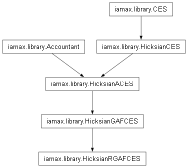

s/e.

aggregated_input_volumes_rooter(self, *, output_volume: np.ndarray, input_volumes: np.ndarray)¶

s/e., \(1 \times 1\) unit-dimensionless zero.

(197)¶\[\approx 0\]

Parameters

output_volume (float) – \(q_j\), i.e. the \(j\)th \(1 \times 1\) output_volumes’s element.
input_volumes (numpy.ndarray) – \((\bQ_{k,j})_{k \in \mcI_j}\), i.e. the \(j\)th \(1 \times |\mcI_j|\) input_volumes’s slice.

See also

aggregated_input_volumes.

class iamax.library.HicksianFLUMRS(*args, **kwargs)¶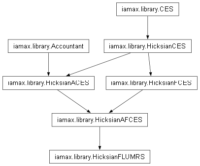: Unit MRS linear (forced) production function which boils down to a special case of HicksianFCES where \(a_k=1 \text{ for } k \in \mcI_j\) and \(\sigma \longrightarrow \infty\).

Note

This class’s compute_calibrand_0() has no system-dependence since the underlying calibrands are inherently equal to \(1\).

class iamax.library.MarshallianCES(*args, **kwargs)¶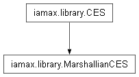

Inheritance diagram of iamax.library.MarshallianCES

Constant Elasticity of Substitution abstraction whose optimal demand function derives from a maximization program formulated à la Marshall.

Note

Calculations assert constant return to scale, i.e. Eq.187’s \(\nu\) is forced to be \(1\) at instantiation.

compute_calibrand_0(self, *, budget_constraint: float, input_values: np.ndarray)¶

Calibrate the \((a_{k,j})_{k \in \mcI_j}\), i.e. the \(|\mcI_j|\) demand share parameters related to aggregate \(j\), considering them equal to the budget share of each of the underlying consumptions in the base year.

(198)¶\[a_k = \frac{\mcv_k}{r_j}, \ \forall k \ \in \mcI_j\]

with \(r_j\) the budget constraint to be saturated, \(\mcI_j\) the index set of the subject-to-\(r_j\) traded off consumptions, \(\mcv_k\) the \(q_k\)’s corresponding input value.

Parameters

budget_constraint (float) – \(r_j\), i.e. the \(j\)th \(1 \times 1\) budget_constraints’s element.
input_values (numpy.ndarray) – \((\bmcV_{k,j})_{k \in \mcI_j}\), i.e. the \(j\)th \(1 \times |\mcI_j|\) input_values’s slice.

Example

>>> m = MarshallianCES(sigma=None)
>>> _ = m.compute_calibrand_0(
...     budget_constraint=200.,
...     input_values=np.array([[110., 90.]])
... )
>>> m._shares_sum
array([[1.]])
>>> m.calibrand_0
array([[0.55, 0.45]])

>>> _ = m.compute_calibrand_0(
...     budget_constraint=100.,
...     input_values=np.array([[110., 90.]])
... )
>>> m._shares_sum
array([[2.]])
>>> m.calibrand_0
array([[0.55, 0.45]])

See also

compute_calibrand_0().

budget_constraint_crooter(self)¶

compute_calibrand_0()’s companion unit-dimensionless zero aiming at ensuring that the sum of shares add up to 1, \(1 \times 1\).

Example

>>> budc  = 200.
>>> ivals = np.array([[110., 90.]])
>>> m = MarshallianCES(sigma=None)
>>> _ = m.compute_calibrand_0(
...     budget_constraint=budc, input_values=ivals
... )
>>> m.budget_constraint_crooter()
array([[0.]])

Let’s then illustrate how such calculation can be vectorized.

>>> vbudc  = np.array([[[.5*budc]], [[budc]], [[2*budc]]])
>>> vivals = np.stack((ivals, ivals, ivals))
>>> m.compute_calibrand_0(
...     budget_constraint=vbudc, input_values=vivals
... ).budget_constraint_crooter()
array([[[ 1. ]],
       [[ 0. ]],
       [[-0.5]]])

input_volumes_computer(self, *, budget_constraint: float, input_prices: np.ndarray)¶

Input demands, \(1 \times |\mcI_j|\), denoted as

(199)¶\[q_k = \frac{ r_j p_{k}^{\frac{1}{\rho_j - 1}} }{ \sum_{k^{'} \in \mcI_j} p_{k^{'}}^{\frac{\rho_j}{\rho_j - 1}} \left[ \frac{a_k}{a_{k^{'}}} \right]^{\frac{1}{\rho_j - 1}} } = \frac{r_j}{ p_{k}^{\sigma_j} \sum_{k^{'} \in \mcI_j} p_{k^{'}}^{1-\sigma_j} \left[ \frac{a_{k^{'}}}{a_{k}} \right]^{\sigma_j} } \ \forall k \ \in \mcI_j\]

where \(r_j\) is the budget constraint to be saturated, \(\rho_j = \frac{\sigma_j - 1}{\sigma_j}\) the substitution parameter, \(\sigma_j = \frac{1}{1 - \rho_j}\) the elasticity of substitution, \(\mcI_j\) the index set of consumptions traded off under \(r_j\), \(p_k\) the \(q_k\)’s price and \(a_k\) as in Eq.198.

What happens internally, is actually performed in matrix terms (so as to benefit from vectorization) as follows:

(200)¶\[\bq = \frac{r_j}{ \bp^{\sigma_j} \odot \mathbf{1}_{|\mcI_j|} \left( \bp^{1 - \sigma_j} \odot \left[ \ba \cdot \frac{1}{\ba^{'}} \right]^{\sigma_j} \right)^{'} }\]

where \(\mathbf{1}_{|\mcI_j|}\), \(\bq = (q_1, \ldots, q_{|\mcI_j|})\), \(\ba = (a_1, \ldots, a_{|\mcI_j|})\) and \(\bp = (p_1, \ldots, p_{|\mcI_j|})\) are \(1 \times |\mcI_j|\) vectors.

Parameters

budget_constraint (float) – \(r_j\), i.e. the \(j\)th \(1 \times 1\) budget_constraints’s element.
input_prices (numpy.ndarray) – \((\tbP_{k,j})_{k \in \mcI_j}\), i.e. the \(j\)th \(1 \times |\mcI_j|\) input_prices’s slice.

Example

Let’s directly deal with the \(\rho_j=0 \iff \sigma_j=1\) CES’s limiting case, which makes it boil down down to a Cobb-Douglas function.

>>> budc  = 200.
>>> ivals = np.array([[110., 90.]])
>>> iprcs = np.array([[.9, 1.1]])

>>> m = MarshallianCES(sigma=1)
>>> _ = m.compute_calibrand_0(
...     budget_constraint=budc, input_values=ivals
... )
>>> m.calibrand_0
array([[0.55, 0.45]])

>>> m.input_volumes_computer(
...     budget_constraint=budc, input_prices=np.ones_like(ivals),
... )
array([[110.,  90.]])
>>> m.input_volumes_computer(
...     budget_constraint=budc, input_prices=iprcs,
... )
array([[122.22,  81.82]])

You can check for yourself via, say, there. Let’s then illustrate how such calculation can be vectorized.

>>> vbudc  = np.array([[[.5*budc]], [[budc]], [[2*budc]]])
>>> vivals = np.stack((ivals, ivals, ivals))
>>> viprcs = np.stack((iprcs, iprcs, iprcs))

>>> m = MarshallianCES(sigma=[[[2.]], [[1.]], [[.5]]])
>>> _ = m.compute_calibrand_0(
...     budget_constraint=vbudc, input_values=vivals
... )
>>> m.calibrand_0
array([[[0.55, 0.45]],
       [[0.55, 0.45]],
       [[0.55, 0.45]]])
>>> m.input_volumes_computer(
...     budget_constraint=vbudc, input_prices=viprcs,
... )
array([[[ 71.79,  32.17]],
       [[122.22,  81.82]],
       [[222.22, 181.82]]])

class iamax.library.MarshallianGFCES(*args, negated_mask: bool = False, **kwargs)¶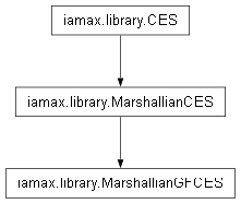

Inheritance diagram of iamax.library.MarshallianGFCES

MarshallianCES’s altered version whose underlying trade-off is forced in a generalized manner by restricting it to a consumption subset of arbitrary size.

Parameters: negated_mask (bool) – Whether the mask passed as argument input_volumes_drates2 of the method compute_calibrand_0 is to be negated. Argument input_volumes_drates2 indeed boolean-specifies the good being subject to consumption tradeoff by default. Set to False by default.

compute_calibrand_0(self, *, budget_constraint: float, input_values: np.ndarray, input_volumes_drates2: np.ndarray)¶

s/e.

Parameters

budget_constraint (float) – \(r_j\), i.e. the \(j\)th \(1 \times 1\) budget_constraints’s element.
input_values (numpy.ndarray) – \((\bmcV_{k,j})_{k \in \mcI_j}\), i.e. the \(j\)th \(1 \times |\mcI_j|\) input_values’s slice.
input_volumes_drates2 (numpy.ndarray) – \((\bQ^\text{drate}_{k,j})_{k \in \mcI_j}\), i.e. the \(j\)th \(1 \times |\mcI_j|\) input_volumes_drates2’s slice. This variable is coerced into boolean and used as mask.

Example

>>> m = MarshallianGFCES(sigma=None, negated_mask=False)
>>> m.compute_calibrand_0(
...     budget_constraint     = 200.,
...     input_values          = np.array([[110., 90.]]),
...     input_volumes_drates2 = np.array([[1., 1.]])
... )
>>> m._shares_sum
array([[1.]])
>>> m.calibrand_0
array([[0.55, 0.45]])

>>> m.compute_calibrand_0(
...     budget_constraint     = 200.,
...     input_values          = np.array([[110., 90.]]),
...     input_volumes_drates2 = np.array([[1., 0.]])
... )
>>> m._shares_sum
array([[1.]])
>>> m.calibrand_0
array([[1., 0.]])

>>> m = MarshallianGFCES(sigma=None, negated_mask=True)
>>> m.compute_calibrand_0(
...     budget_constraint     = 200.,
...     input_values          = np.array([[110., 90.]]),
...     input_volumes_drates2 = np.array([[0., 0.]])
... )
>>> m._shares_sum
array([[1.]])
>>> m.calibrand_0
array([[0.55, 0.45]])

>>> m.compute_calibrand_0(
...     budget_constraint     = 200.,
...     input_values          = np.array([[110., 90.]]),
...     input_volumes_drates2 = np.array([[1., 0.]])
... )
>>> m._shares_sum
array([[1.]])
>>> m.calibrand_0
array([[0., 1.]])

See also

compute_calibrand_0().

input_volumes_computer(self, budget_constraint: float, input_values: np.ndarray, input_prices: np.ndarray)¶

s/e.

Parameters

budget_constraint (float) – \(r_j\), i.e. the \(j\)th \(1 \times 1\) budget_constraints’s element.
input_values (numpy.ndarray) – \((\bmcV_{k,j})_{k \in \mcI_j}\), i.e. the \(j\)th \(1 \times |\mcI_j|\) input_values’s slice.
input_prices (numpy.ndarray) – \((\tbP_{k,j})_{k \in \mcI_j}\), i.e. the \(j\)th \(1 \times |\mcI_j|\) input_prices’s slice.

Example

Let’s directly deal with the \(\rho_j=0 \iff \sigma_j=1\) CES’s limiting case, which makes it boil down down to a Cobb-Douglas function.

>>> budc  = 200.
>>> ivals = np.array([[110., 90.]])
>>> iprcs = np.array([[.9, 1.1]])

>>> imsks = np.array([[1., 0.]])
>>> m = MarshallianGFCES(sigma=1, negated_mask=False)
>>> m.compute_calibrand_0(
...     budget_constraint=budc, input_values=ivals,
...     input_volumes_drates2=imsks
... )
>>> m.calibrand_0
array([[1., 0.]])
>>> m.input_volumes_computer(
...     budget_constraint=budc, input_prices=np.ones_like(ivals),
...     input_values=ivals,
... )
array([[110.,  90.]])
>>> m.input_volumes_computer(
...     budget_constraint=budc, input_prices=iprcs,
...     input_values=ivals,
... )
array([[122.22,  81.82]])

>>> imsks = np.array([[0., 1.]])
>>> m = MarshallianGFCES(sigma=1, negated_mask=True)
>>> m.compute_calibrand_0(
...     budget_constraint=budc, input_values=ivals,
...     input_volumes_drates2=imsks
... )
>>> m.calibrand_0
array([[1., 0.]])
>>> m.input_volumes_computer(
...     budget_constraint=budc, input_prices=np.ones_like(ivals),
...     input_values=ivals,
... )
array([[110.,  90.]])
>>> m.input_volumes_computer(
...     budget_constraint=budc, input_prices=iprcs,
...     input_values=ivals,
... )
array([[122.22,  81.82]])

See also

input_volumes_computer().

spendings_rooter(self, *, budget_constraint: float, input_values: np.ndarray)¶

s/e., \(1 \times 1\) unit-dimensionless zero.

(201)¶\[\approx 0\]

Parameters

budget_constraint (float) – \(r_j\), i.e. the \(j\)th \(1 \times 1\) budget_constraints’s element.
input_values (numpy.ndarray) – \((\bmcV_{k,j})_{k \in \mcI_j}\), i.e. the \(j\)th \(1 \times |\mcI_j|\) input_values’s slice.

class iamax.library.MarshallianLeo¶

Inheritance diagram of iamax.library.MarshallianLeo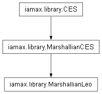

Particularized version of MarshallianCES at \(\sigma=0\).

Warning

This class has vocation to be removed sooner or later and obtained directly through the parametrization of MarshallianCES.

compute_calibrand_0(self, *, input_prices: np.ndarray, input_volumes: np.ndarray)¶

s/e.

(202)¶\[a_k = q_k / \sum_{k^{'} \in \mcI_j} q_{k^{'}} \ \forall k \ \in \mcI_j\]

where \(q_k\) is the utility maximizing level of consumption.

Parameters

input_prices (numpy.ndarray) – \((\tbP_{k,j})_{k \in \mcI_j}\), i.e. the \(j\)th \(1 \times |\mcI_j|\) input_prices’s slice.
input_volumes (numpy.ndarray) – \((\bQ_{k,j})_{k \in \mcI_j}\), i.e. the \(j\)th \(1 \times |\mcI_j|\) input_volumes’s slice.

Example

>>> m = MarshallianLeo()
>>> _ = m.compute_calibrand_0(
...     input_prices=np.ones((1, 2)),
...     input_volumes=np.array([[110., 90.]])
... )
>>> m.calibrand_0
array([[0.55, 0.45]])

input_volumes_computer(self, *, budget_constraint: float, input_prices: np.ndarray, **_: np.ndarray)¶

Input demands, \(1 \times |\mcI_j|\), denoted as

(203)¶\[q_k = a_k \frac{r_j}{ \sum_{k^{'} \in \mcI_j} \tbp_{k^{'}} a_{k^{'}} } \ \forall k \ \in \mcI_j\]

where \(r_j\) is the budget constraint to be saturated, \(a_k\) is as in Eq.202 and \(\tbp_k\) is the \(k\)th price of consumption.

Parameters

budget_constraint (float) – \(r_j\), i.e. a \(j\)-related \(1 \times 1\) budget_constraints’s element.
input_prices (numpy.ndarray) – \((\tbP_{k,j})_{k \in \mcI_j}\), i.e. the \(j\)th \(1 \times |\mcI_j|\) input_prices’s slice.

Example

>>> m = MarshallianLeo()
>>> _ = m.compute_calibrand_0(
...     input_prices=np.array([[1.01, .99]]),
...     input_volumes=np.array([[110., 90.]])
... )
>>> m.calibrand_0
array([[0.55, 0.45]])
>>> m.input_volumes_computer(
...     budget_constraint=200, input_prices=np.ones((1, 2)),
... )
array([[110.,  90.]])

class iamax.library.EmplBMagnitude¶

Static class that aggregates a bunch of private methods related to employment- and utilization-based magnitudes.

static _drate_pow_increaser(*, dr: float, c: float = 1.0, s: float = 1.0)¶

Rate differential increasing function.

(204)¶\[\mfr(dr, c, s) := s\left(1 + dr\right)^{c}\]

Cf. parameters section below.

Parameters

dr (float) – Underlying rates differential of interest.
c (float) – Magnitude exponentiation parameter. To 1. by default.
s (float) – Scale factor (and value at \(dr=0\)). To 1. by default.

Note

For \(c < 0\), the function turns \(dr\)-decreasing.

Example

>>> invariants = {'c': .2, 's': 1.}
>>> EmplBMagnitude._drate_pow_increaser(dr=-.5, **invariants)
0.8705505632961241
>>> EmplBMagnitude._drate_pow_increaser(dr=.0, **invariants)
1.0
>>> EmplBMagnitude._drate_pow_increaser(dr=.5, **invariants)
1.0844717711976986

static _factor_pow_increaser(*, f: float, c: float = 1.0, s: float = 1.0)¶

Factor increasing function.

(205)¶\[\mfr(f, c, s) := s f^c\]

Parameters

f (float) – Underlying 1-centered factor e.g. rates ratio.
c (float) – Magnitude exponentiation parameter. To 1. by default.
s (float) – Scale factor (and value at \(f=1\)). To 1. by default.

Note

For \(c < 0\), the function turns \(f\)-decreasing.

Example

>>> invariants = {
...     'c': .2,
...     's': 1.,
... }
>>> EmplBMagnitude._factor_pow_increaser(f=.5, **invariants)
0.8705505632961241
>>> EmplBMagnitude._factor_pow_increaser(f=1.0, **invariants)
1.0
>>> EmplBMagnitude._factor_pow_increaser(f=1.5, **invariants)
1.0844717711976986
>>> EmplBMagnitude._factor_pow_increaser(f=-.5, **invariants)
0.7042902001692477

static _rate_tanh_increaser(*, r: float, a: float = 1.0, b: float = 1.0, c: float = 1.0, s: float = 1.0)¶

Rate increasing function.

(206)¶\[\mfr(r, a, b, c, s) := s\left( a + b \tanh(-c r) \right)\]

Cf. parameters section below.

Parameters

r (float) – Underlying rate of interest.
a (float) – Magnitude upper bound. To 1. by default.
b (float) – Magnitude lower bound parameter. To 1. by default.
c (float) – Magnitude sigmoid parameter. To 1. by default.
s (float) – Scale factor. To 1. by default.

Note

For \(c < 0\), the order of \(a\) and \(b\) is reversed, i.e. the function turns \(r\)-decreasing.

Example

>>> invariants = {
...     'a': .05,
...     'b': .711594155955765,
...     'c': 1.09045112440194,
...     's': 1.
... }
>>> EmplBMagnitude._rate_tanh_increaser(r=.0, **invariants)
0.05
>>> EmplBMagnitude._rate_tanh_increaser(r=.5, **invariants)
-0.3036148489085014
>>> EmplBMagnitude._rate_tanh_increaser(r=1., **invariants)
-0.5171709549513277

class iamax.library.PowCurvedNetPrice(sigma: float|np.ndarray, urate_bias: float|np.ndarray = 0.0)¶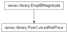

Inheritance diagram of iamax.library.PowCurvedNetPrice

Net-price curve abstraction, whose name stems from the generalization of the well vertued negative relationship between wages and local unemployment, a.k.a. the wage curve.

Parameters

sigma (float) – Elasticity of price with respect to the difference between an unemployment reference- and running-rate.
urate_bias (float) – Parameter that allows unemployment reference- and running-rates to be shifted to the left or right. Set to .0 by default.

Note

Such elasticity is assumed to measure the sensitivity of prices to changes in market conditions relative to a specific baseline, rather than simply the level of unemployment.

compute_calibrand_0(self, *, output_price: np.float|np.ndarray, unemployment_rate: np.float|np.ndarray)¶

Curve parametrization, performed such that

(207)¶\[\begin{split}\up^{*}_j &= \up_{j,t=0} \\ \tau_{\neg\hq, j}^{*} &= \tau_{\neg\hq, j,t=0}\end{split}\]

where \(\up_{j,t=0}\) is the (producer net) price at \(t=0\) and \(\tau_{\neg\hq, j,t=0}\) the rate of unemployed capacity at \(t=0\).

Parameters

output_price (float) – \(\up_j\), i.e. the \(j\)th \(1 \times 1\) output_prices’s element.
unemployment_rate (float) – \(\tau_{\neg\hq, j}\), i.e. the \(j\)th \(1 \times 1\) unemployment_rates’s element.

Example

>>> cnp = PowCurvedNetPrice(sigma=None)
>>> cnp.compute_calibrand_0(
...     output_price=1e2, unemployment_rate=.1
... )
>>> cnp.price_ref
100.0
>>> cnp.price_ref_star
100.0
>>> cnp.urate_ref
0.1
>>> cnp.urate_bias
0.0

compute_calibrand_0_star(self, *, deflators_fisher_drates: np.ndarray)¶

Parameters: deflators_fisher_drates (numpy.ndarray) – \((\bmfp^{\text{drate}}_{\text{F}, k})_{k \in \mcI_j}\), i.e. a \(j\)th \(1 \times 2\) slice of deflators_fisher_drates, whose second component is of interest.

output_price_computer(self, *, unemployment_rate: float, deflators_fisher: np.ndarray, output_price_drate: np.ndarray = 0.0, output_price_drate2: np.ndarray = 0.0)¶

s/e., \(1 \times 1\), denoted as

(208)¶\[\begin{split}\up_j &= \up^{*}_j ( 1 + \up^{\text{drate}}_j + \up^{\text{drate}^{ii}}_j ) \mfp_{\text{F}, j} \left( \frac{\tau_{\neg\hq, j}^{*} + b}{\tau_{\neg\hq, j} + b} \right)^{\sigma_j} \\ &= \mfr\left( s=\up^{*}_j ( 1 + \up^{\text{drate}}_j + \up^{\text{drate}^{ii}}_j ) \mfp_{\text{F}, j}, c=\sigma_j, f=\frac{\tau_{\neg\hq, j}^{*} + b}{\tau_{\neg\hq, j} + b} \right)\end{split}\]

where the star superscript, i.e. \(.^{*}\), and the \(j\) subscript, i.e. \(._{j}\), respectively stand for the idea of “reference” and that of being \(j\)th, \(\up\) is the (producer net) price, \(\tau_{\neg\hq}\) is the rate of unemployment, \(\sigma\) is the elasticity of \(\up\) to (what turns out to be) a rates ratio, \(b\) is a bias parameter, \(\mfp_{\text{F}}\) is the (chained) Fisher deflator and \(\mfr(.)\) is the function detailed in Eq.205.

Reference:: This formulation is taken (and particularized) from KLEM’s equation 12b, the consumer price index put aside.

Parameters

unemployment_rate (float) – \(\tau_{\neg\hq, j}\), i.e. the \(j\)th \(1 \times 1\) unemployment_rates’s element.
deflators_fisher (numpy.ndarray) – \((\bmfp_{\text{F}, k})_{k \in \mcI_j}\), i.e. a \(j\)th \(1 \times 2\) slice of deflators_fisher, whose first component is of interest.
output_price_drate (numpy.ndarray) – \(\up^{\text{drate}}_j\), i.e. the \(j\)th \(1 \times 1\) producer_net_prices_drates’s element. Set to .0 by default.
output_price_drate2 (numpy.ndarray) – \(\up^{\text{drate}^{ii}}_j\), i.e. the \(j\)th \(1 \times 1\) producer_net_prices_drates2’s element. Set to .0 by default.

Important

This method relies on the structure of its argument, as outlined in the description of argument deflators_fisher.

Example

>>> cnp = PowCurvedNetPrice(sigma=.2)
>>> cnp.compute_calibrand_0(
...     output_price=100, unemployment_rate=.1
... )
>>> cnp.output_price_computer(
...     unemployment_rate = .1490099501,
...     deflators_fisher  = np.array([[1.07220603770351, np.nan]])
... )
array([[99.]])
>>> cnp.output_price_computer(
...     unemployment_rate = .0489899499000005,
...     deflators_fisher  = np.array([[0.87567464071516, np.nan]])
... )
array([[101.]])

class iamax.library.TanhCurvedNetPrice(a: float, b: float, c: float)¶

Inheritance diagram of iamax.library.TanhCurvedNetPrice

Yet another net-price curve abstraction.

Parameters

a (float) – Unscaled price lower bound (for c < 0).
b (float) – Unscaled price upper bound parameter (for c < 0).
c (float) – Unscaled price sigmoid parameter.

compute_calibrand_0(self, *, output_price: float, deflators_fisher: np.ndarray)¶

Curve parametrization, performed such that

(209)¶\[\begin{split}\up^{*}_j &= \up_{j,t=0} \\ \mfp_{\text{F}, j}^{*} &= \mfp_{\text{F}, j,t=0}\end{split}\]

where \(\up_{j,t=0}\) is the (producer net) price at \(t=0\) and \(\mfp_{\text{F}, j,t=0}\) the \(j\)-relevant (chained) Fisher price index at \(t=0\).

Parameters

output_price (float) – \(\up_j\), i.e. the \(j\)th \(1 \times 1\) output_prices’s element.
deflators_fisher (numpy.ndarray) – \((\bmfp_{\text{F}, k})_{k \in \mcI_j}\), i.e. a \(j\)th \(1 \times |\mcI_j|\) slice of deflators_fisher, whose first component only is of interest, keeping in mind that \(|\mcI_j|\) is asserted to be equal to \(2\).

Important

This method relies on the structure of its argument, as outlined in the description of argument deflators_fisher.

Example

>>> cnp = TanhCurvedNetPrice(a=None, b=None, c=None)
>>> cnp.compute_calibrand_0(
...     output_price=943.5509, deflators_fisher=np.array(
...         [[1.13748, np.nan]]
...     )
... )
>>> cnp._reference_price
943.5509
>>> cnp._reference_index
array([[1.14]])
>>> cnp.reference_real_price
array([[829.51]])

output_price_computer(self, *, unemployment_rate: float, deflators_fisher: np.ndarray, deflators_fisher_drates: np.ndarray)¶

s/e., \(1 \times 1\).

(210)¶\[\begin{split}\up_j &= \up^{*}_j \frac{ \mfp_{\text{F}, j} }{ \mfp_{\text{F}, j}^{*} }\left( a + b \tanh(-c \tau_{\neg\hq, j}) \right) \\ &= \mfr\left( r=\tau_{\neg\hq, j}, a=a, b=b, c=c, s=\up^{*}_j \frac{ \mfp_{\text{F}, j} }{ \mfp_{\text{F}, j}^{*} } \right)\end{split}\]

where the star superscript, i.e. \(.^{*}\), and the \(j\) subscript, i.e. \(._{j}\), respectively stand for the idea of of “reference” and that of being \(j\)th, \(\up\) is the (producer net) price, \(\tau_{\neg\hq}\) is the rate of unemployment, \(\mfp_{\text{F}}\) is the (chained) Fisher deflator and \(\mfr(.)\) is the function detailed in Eq.206.

Parameters

unemployment_rate (float) – \(\tau_{\neg\hq, j}\), i.e. the \(j\)th \(1 \times 1\) unemployment_rates’s element.
deflators_fisher (numpy.ndarray) – \((\bmfp_{\text{F}, k})_{k \in \mcI_j}\), i.e. a \(j\)th \(1 \times 2\) slice of deflators_fisher, whose first component is of interest.
deflators_fisher_drates (numpy.ndarray) – \((\bmfp^{\text{drate}}_{\text{F}, k})_{k \in \mcI_j}\), i.e. a \(j\)th \(1 \times 2\) slice of deflators_fisher_drates, whose first component is of interest.

Example

Some unscaled examples first.

>>> invariant0 = {'deflators_fisher': np.array([[1., np.nan]])}
>>> invariant  = {
...     **invariant0, 'deflators_fisher_drates': np.zeros((1, 2))
... }

A rate-decreasing case first, whose results belong to \([-b + a, \ a]\).

>>> cnp = TanhCurvedNetPrice(a=.01, b=1, c=1)
>>> cnp.compute_calibrand_0(output_price=1., **invariant0)
>>> cnp.output_price_computer(unemployment_rate=.0, **invariant)
array([[0.01]])
>>> cnp.output_price_computer(unemployment_rate=.5, **invariant)
array([[-0.45]])
>>> cnp.output_price_computer(unemployment_rate=1., **invariant)
array([[-0.75]])

Let’s turn it rate-increasing over \([a, \ b + a]\)

>>> cnp.c *= -1
>>> cnp.output_price_computer(unemployment_rate=.0, **invariant)
array([[0.01]])
>>> cnp.output_price_computer(unemployment_rate=.5, **invariant)
array([[0.47]])
>>> cnp.output_price_computer(unemployment_rate=1., **invariant)
array([[0.77]])

Yet another (scaled) example.

>>> cnp = TanhCurvedNetPrice(
...     a=0, b=2, c=-12.5160928423905
... )
>>> p0 = 943.5508481986847
>>> d0 = np.array([[1.1374749692500363, np.nan]])
>>> cnp.compute_calibrand_0(output_price=p0, deflators_fisher=d0)
>>> r = .05
>>> d = np.array([[1.1280702850130508, np.nan]])
>>> cnp.output_price_computer(
...     unemployment_rate=r, deflators_fisher=d,
...     deflators_fisher_drates=np.zeros((1, 2))
... )
array([[1038.98]])

Let’s vectorize the above example

>>> cnp = TanhCurvedNetPrice(
...     a=0., b=2., c=np.array([
...         [[cnp.c]], [[cnp.c]], [[-24]]
...     ])
... )
>>> cnp.compute_calibrand_0(
...     deflators_fisher=np.stack((d0, d0, d0)),
...     output_price=np.array([
...         [[p0]], [[.1*p0]], [[p0]]
...     ])
... )
>>> cnp.output_price_computer(
...     deflators_fisher=np.stack((d, d, d)),
...     deflators_fisher_drates=np.zeros((3, 1, 2)),
...     unemployment_rate=np.array([
...         [[r]], [[r]], [[r]]
...     ])
... )
array([[[1038.98]],
       [[ 103.9 ]],
       [[1560.18]]])

class iamax.library.NetPriceTanhCurvedMultiplier(*, a: float, b: float, c: float)¶

Inheritance diagram of iamax.library.NetPriceTanhCurvedMultiplier

Net-price’s multiplier abstraction.

Parameters

a (float) – Multiplier’s upper bound (for c > 0).
b (float) – Multiplier’s lower bound parameter (for c > 0).
c (float) – Multiplier’s sigmoid parameter.

Note

To learn more about the underlying narrative, refer to Bibas et al.’s (2016) IMAClim-R model documentation (version 1.1).

output_price_computer(self, *, input_prices: np.ndarray, idle_rates: np.ndarray)¶

s/e., \(1 \times 1\).

\[\begin{split}\ubp_{j=1} &= \tbp_{j=1} \left( a + b \tanh(-c \left[1 - \btau_{\neg q, 2}\right]) \right) \\ &= \mfr\left( r=1 - \btau_{\neg q, 2}, a=a, b=b, c=c, s=\tbp_{j=1} \right)\end{split}\]

where \(\tbp_{1}\) and \(\btau_{\neg q, 2}\) are respectively the input price and idle rate of interest, scalar, \(\mfr(.)\) is as defined in Eq.206 and \(a\), \(b\), \(c\) (positive) and \(s\) the instantiation parameters.

Parameters

input_prices (numpy.ndarray) – \((\tbP_{k,j})_{k \in \mcI_j}\), i.e. the \(j\)th \(1 \times |\mcI_j|\) slice of input_prices, whose first component only is of interest, keeping in mind that \(|\mcI_j|\) is asserted to be equal to \(2\).
idle_rates (numpy.ndarray) – \((\btau_{\neg q, k})_{k \in \mcI_j}\), i.e. a \(j\)th \(1 \times 2\) slice of idle_rates, whose second component only is of interest.

Important

As outlined in the parameters’ descriptions, the current method relies on the structure of its arguments.

Example

>>> npcm = NetPriceTanhCurvedMultiplier(
...     a=1.05, b=0.1008758, c=2.7176754
... )
>>> npcm.output_price_computer(**(ut1 := dict(
...     input_prices = np.array([[1., np.nan]]),
...     idle_rates   = np.array([[np.nan, .0]]),
... )))
array([[1.05]])
>>> npcm.output_price_computer(**(ut2 := dict(
...     input_prices = np.array([[1., np.nan]]),
...     idle_rates   = np.array([[np.nan, .5]]),
... )))
array([[0.96]])
>>> npcm.output_price_computer(**(ut3 := dict(
...     input_prices = np.array([[1., np.nan]]),
...     idle_rates   = np.array([[np.nan, 1.]]),
... )))
array([[0.95]])

Let’s find the idle rate that puts output prices to 1.

>>> from scipy import optimize as sop
>>> x = sop.minimize(
...     tol=1e-30, x0=[0.], fun=lambda x: np.array([
...         -1 + npcm.output_price_computer(
...             input_prices = np.array([[1., np.nan]]),
...             idle_rates   = np.array([[np.nan, x[0]]])
...         )
...     ])**2
... ).x.item()
>>> x
0.1999998919765992
>>> npcm.output_price_computer(**(ut4 := dict(
...     input_prices = np.array([[1., np.nan]]),
...     idle_rates   = np.array([[np.nan, x]]),
... ))).item()
1.0000000015407478

Another (less conservative) example.

>>> npcm._precomp = {'a': 30., 'b': 29.2, 'c': 14.183308}
>>> npcm.output_price_computer(**ut1).item()
30.0
>>> npcm.output_price_computer(**ut2).item()
0.8000404278035766
>>> npcm.output_price_computer(**ut3).item()
0.800000000027989
>>> npcm.output_price_computer(**ut4).item()
1.000000624142121

class iamax.library.TanhCMultipliedTanhCNetPrice(*, p_a: float, p_b: float, p_c: float, m_a: float, m_b: float, m_c: float)¶

Multiplied net-price curve abstraction.

Parameters

p_a (float) – Unscaled price lower bound (for p_c < 0).
p_b (float) – Unscaled price upper bound parameter (for p_c < 0).
p_c (float) – Unscaled price sigmoid parameter.
m_a (float) – Multiplier’s upper bound (for m_c > 0).
m_b (float) – Multiplier’s lower bound parameter (for m_c > 0).
m_c (float) – Multiplier’s sigmoid parameter.

Note

This class internally makes use of TanhCurvedNetPrice and NetPriceTanhCurvedMultiplier through composition.

Example

>>> o = TanhCMultipliedTanhCNetPrice(
...     p_a=None, p_b=None, p_c=None,
...     m_a=None, m_b=None, m_c=None,
... )
>>> o.pricecurve.__class__.__name__
'TanhCurvedNetPrice'
>>> o.multiplier.__class__.__name__
'NetPriceTanhCurvedMultiplier'

compute_calibrand_0(self, *, output_price: float, deflators_fisher: np.ndarray)¶

Curve parametrization, performed as explained in Eq.209.

Note

This method internally resort to compute_calibrand_0().

Parameters

output_price (float) – \(\up_j\), i.e. the \(j\)th \(1 \times 1\) output_prices’s element.
deflators_fisher (numpy.ndarray) – \((\bmfp_{\text{F}, k})_{k \in \mcI_j}\), i.e. a \(j\)th \(1 \times |\mcI_j|\) slice of deflators_fisher, whose first component only is of interest, keeping in mind that \(|\mcI_j|\) is asserted to be equal to \(3\).

Important

This method relies on the structure of its argument, as outlined in the description of argument deflators_fisher.

Example

>>> o = TanhCMultipliedTanhCNetPrice(
...     **dict.fromkeys([
...         'p_a', 'p_b', 'p_c',
...         'm_a', 'm_b', 'm_c',
...     ])
... )
>>> o.compute_calibrand_0(
...     output_price=943.55, deflators_fisher=np.array(
...         [[1.14, np.nan, np.nan]]
...     )
... )
>>> (cnp := o.pricecurve)._reference_price
943.55
>>> cnp._reference_index
array([[1.14]])
>>> cnp.reference_real_price
array([[827.68]])

output_price_computer(self, *, unemployment_rate: float, idle_rates: float, deflators_fisher: np.ndarray, deflators_fisher_drates: np.ndarray)¶

s/e., \(1 \times 1\).

Parameters

unemployment_rate (numpy.ndarray) – \(\btau_{\neg \hq, j}\), i.e. the \(j\)th \(1 \times 1\) unemployment_rates’s element.
idle_rates (numpy.ndarray) – \((\btau_{\neg q, k})_{k \in \mcI_j}\), i.e. a \(j\)th \(1 \times 3\) slice of idle_rates, whose third component only is of interest.
deflators_fisher (numpy.ndarray) – \((\bmfp_{\text{F}, k})_{k \in \mcI_j}\), i.e. a \(j\)th \(1 \times 3\) slice of deflators_fisher, whose first component is of interest.
deflators_fisher_drates (numpy.ndarray) – \((\bmfp^{\text{drate}}_{\text{F}, k})_{k \in \mcI_j}\), i.e. a \(j\)th \(1 \times 3\) slice of deflators_fisher_drates, whose first component is of interest.

Example

>>> o = TanhCMultipliedTanhCNetPrice(
...     p_a=0, p_b=2, p_c=-12.5160928423905,
...     m_a=1.05, m_b=0.1008758, m_c=2.7176754,
... )
>>> o.compute_calibrand_0(
...     output_price     = 943.55085,
...     deflators_fisher = np.array([[1.13748]])
... )
>>> o.output_price_computer(
...     unemployment_rate       = .05,
...     idle_rates              = np.array([[np.nan, .5]]),
...     deflators_fisher        = np.array([[1.12807]]),
...     deflators_fisher_drates = np.zeros((1, 1))
... )
array([[999.09]])

class iamax.library.LaborMarket¶: s/e.

class iamax.library.UniformProductivityPremia¶

Uniformly solved productivity premia.

static output_volume_rooter(ioq_productivities_drates2: np.ndarray)¶

s/e., \(1 \times 1\) zero(s).

Parameters

ioq_productivities_drates2 (numpy.ndarray) – \((\balpha^{-1,\ \text{drate}_{kk,j}})_{k \in \mcI_j}\), i.e. the \(j\)th \(|\mcI_j| \times |\mcI_j|\) ioq_productivities_drates2’s (diagonal) square slice.

Example

>>> a = np.array([0, 1., .2]) * np.identity(3)
>>> UniformProductivityPremia.output_volume_rooter(
...     ioq_productivities_drates2=a
... )
array([[0.71, 0.71, 0.71]])

Let’s vectorize the above example.

>>> (v := np.stack((a, np.identity(3))))
array([[[0. , 0. , 0. ],
        [0. , 1. , 0. ],
        [0. , 0. , 0.2]],
       [[1. , 0. , 0. ],
        [0. , 1. , 0. ],
        [0. , 0. , 1. ]]])
>>> UniformProductivityPremia.output_volume_rooter(
...     ioq_productivities_drates2=v
... )
array([[[0.71, 0.71, 0.71]],
       [[0.  , 0.  , 0.  ]]])

class iamax.library.UniformGhoshAllocationPremia¶

Uniformly solved GhoshAllocation premia.

static output_volume_rooter(ioq_shares_drates2: np.ndarray)¶

s/e., \(1 \times 1\) zero(s).

Parameters

ioq_shares_drates2 (numpy.ndarray) – \((\bbeta^{\text{drate}^{ii}}_{kk,j})_{k \in \mcI_j}\), i.e. the \(j\)th \(|\mcI_j| \times |\mcI_j|\) ioq_shares_drates2’s slice.

Example

>>> a = np.array([0, 1., .2]) * np.identity(3)
>>> UniformGhoshAllocationPremia.output_volume_rooter(
...     ioq_shares_drates2=a
... )
array([[0.71, 0.71, 0.71]])

Let’s vectorize the above example.

>>> (v := np.stack((a, np.identity(3))))
array([[[0. , 0. , 0. ],
        [0. , 1. , 0. ],
        [0. , 0. , 0.2]],
       [[1. , 0. , 0. ],
        [0. , 1. , 0. ],
        [0. , 0. , 1. ]]])
>>> UniformGhoshAllocationPremia.output_volume_rooter(
...     ioq_shares_drates2=v
... )
array([[[0.71, 0.71, 0.71]],
       [[0.  , 0.  , 0.  ]]])

class iamax.library.UniformPrice(price_transmitting: bool = False)¶

Uniformly equalized prices.

Parameters: price_transmitting (bool) – Whether the price of the aggregate is to be granularly communicated. Set to False by default.

compute_calibrand_0(self, *, output_volumes: np.ndarray, t: int = 0)¶

Ancillary method whose only goal is to compute the mask that specifies which elements are to be included when producer_net_prices_rooter() is called.

Parameters

output_volumes (numpy.ndarray) – \((\ubq_k)_{k \in \mcI_j}\), i.e. a reconstructed slice of output_volumes.
t (int) – Year-targeting integer index. Cf. t, i.e. a _ilocalizations’s integer element. To 0 by default.

Example

>>> a = np.array([
...     [[0, 1., .2, 1.]],
...     [[0, 1., 1., 2.]],
...     [[0, 3., .4, 8.]],
...     [[0, 1., 1., 1.]],
... ])

>>> pt = False
>>> uu = UniformPrice(pt).compute_calibrand_0(
...     output_volumes=a
... )
>>> uu._ix0, uu._trnsm_mask
(1, True)

>>> pt = True
>>> uu = UniformPrice(pt).compute_calibrand_0(
...     output_volumes=a
... )
>>> uu._ix0, uu._trnsm_mask
(0, True)

Let’s vectorize the above example, keeping in mind that the temporal axis must remain first (hence the use of numpy.ndarray.swapaxes below).

>>> v  = np.stack((a + 1, a)).swapaxes(1, 0)
>>> pt = np.array([[[True]], [[False]]])
>>> uu = UniformPrice(pt).compute_calibrand_0(
...     output_volumes=v
... )
>>> uu._ix0
0
>>> uu._trnsm_mask
array([[[[ True,  True,  True,  True]],
        [[False,  True,  True,  True]]]])

producer_net_prices_rooter(self, *, t: int, producer_net_prices: np.ndarray)¶

s/e.

Parameters

t (int) – Year-targeting integer index. Cf. t, i.e. a _ilocalizations’s integer element.
producer_net_prices (numpy.ndarray) – \((\ubp_k)_{k \in \mcI_j}\), i.e. a reconstructed slice of producer_net_prices.

See also

producer_net_prices.

Important

Since it resorts to t, the current method relies on the structure of its non-scalar arguments, as explained here.

Note

This method is vectorization friendly over the -3th axis, if any.

Example

>>> a = np.array([
...     [[0, 1., .2, 1.]],
...     [[0, 1., 1., 2.]],
...     [[0, 3., .4, 8.]],
...     [[0, 1., 1., 1.]],
... ])
>>> UniformPrice().producer_net_prices_rooter(
...     producer_net_prices=a, t=1
... )
array([[[0.23]]])
>>> UniformPrice().producer_net_prices_rooter(
...     producer_net_prices=a, t=2
... )
array([[[0.59]]])
>>> UniformPrice().producer_net_prices_rooter(
...     producer_net_prices=a, t=3
... )
array([[[0.]]])

Let’s vectorize the above example, keeping in mind that the temporal axis must remain first (hence the use of numpy.ndarray.swapaxes below).

>>> (v := np.stack((a + 1, a)).swapaxes(1, 0))
array([[[[1. , 2. , 1.2, 2. ]],
        [[0. , 1. , 0.2, 1. ]]],
       [[[1. , 2. , 2. , 3. ]],
        [[0. , 1. , 1. , 2. ]]],
       [[[1. , 4. , 1.4, 9. ]],
        [[0. , 3. , 0.4, 8. ]]],
       [[[1. , 2. , 2. , 2. ]],
        [[0. , 1. , 1. , 1. ]]]])
>>> UniformPrice().producer_net_prices_rooter(
...     producer_net_prices=v, t=2
... )
array([[[[0.46]],
        [[0.59]]]])
>>> UniformPrice().producer_net_prices_rooter(
...     producer_net_prices=v, t=3
... )
array([[[[0.]],
        [[0.]]]])

class iamax.library.UniformUnemployment¶

Uniformly unemployed capacities.

Note

We may think about labor when reading ‘unemployment’ but this class is absolutely agnostic regarding the very nature of the entities you assign them to.

static unemployment_rates_rooter(t: int, unemployment_rates: np.ndarray)¶

s/e.

See also

unemployment_rates.

Important

Although it resorts to t, the current method does not rely on the structure unemployment_rates, as explained here.

Note

This method is vectorization friendly over the -3th axis, if any.

Example

>>> a = np.array([
...     [[.2, .1, .3]],
...     [[.2, .2, .2]],
... ])
>>> UniformUnemployment.unemployment_rates_rooter(
...     t=0, unemployment_rates=a
... )
array([[[0.3]]])
>>> UniformUnemployment.unemployment_rates_rooter(
...     t=1, unemployment_rates=a
... )
array([[[9.66e-17]]])

Let’s vectorize the above example, keeping in mind that the temporal axis must remain first (hence the use of numpy.ndarray.swapaxes below).

>>> (v := np.stack((a, 2*a)).swapaxes(1, 0))
array([[[[0.2, 0.1, 0.3]],
        [[0.4, 0.2, 0.6]]],
       [[[0.2, 0.2, 0.2]],
        [[0.4, 0.4, 0.4]]]])
>>> UniformUnemployment.unemployment_rates_rooter(
...     t=1, unemployment_rates=v
... )
array([[[[9.66e-17]],
        [[9.77e-17]]]])

class iamax.library.ULaborMarket¶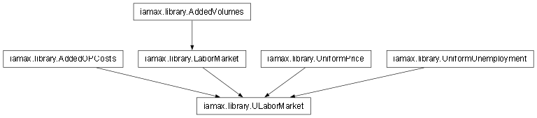: s/e.

class iamax.library.UMarket¶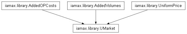: s/e.

class iamax.library.UUMarket¶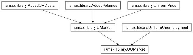: s/e.

class iamax.library.TermsOfTrade(sigma: float)¶

Example case-denominated Terms of Trade.

Parameters: sigma (float) – Elasticity to terms-of-trade of good exports.

compute_calibrand_0(self, *, arent_final: np.ndarray, are_only_final: np.ndarray, specific_producer_prices: np.ndarray, consumer_prices: np.ndarray, ioq_shares: np.ndarray)¶

Support the calibration of the constant scale factor implied in the terms-of-trade equation, denoted as

(211)¶\[A_X = \frac{q_{X(t=0)}}{q_{S(t=0)}} \left( \frac{p_{X(t=0)}}{p_{M(t=0)}} \right)^\sigma\]

where \(q_{X(t=0)}/q_{S(t=0)}\) is the share of exported quantity with respect to that of the Armington aggregate, \(p_{X(t=0)}/p_{M(t=0)}\) the price ratio of the former against its imported counterpart and \(\sigma\) the elasticity to terms-of-trade of good exports, set at instantiation.

Parameters

arent_final (numpy.ndarray) – \((\btxta_k)_{k \in \mcI_j}\), i.e. the \(j\)th \(1 \times |\mcI_j|\) arent_final’s slice.
are_only_final (numpy.ndarray) – \((\textbf{f}_k)_{k \in \mcI_j}\), i.e. a \(j\)-th \(1 \times |\mcI_j|\) are_only_final’s slice.
specific_producer_prices (numpy.ndarray) – \((\tbP^{T}_{k,j})_{k \in \mcI_j}\), i.e. a \(j\)-th \(1 \times |\mcI_j|\) specific_producer_prices’s slice.
consumer_prices (numpy.ndarray) – \((\tbP_{k,j})_{k \in \mcI_j}\), i.e. a \(j\)-th \(1 \times |\mcI_j|\) consumer_prices’s slice.
ioq_shares (numpy.ndarray) – \((\bbeta_{k,j})_{k \in \mcI_j}\), i.e. a \(j\)-th \(1 \times |\mcI_j|\) ioq_shares’s slice.

output_volume_rooter(self, specific_producer_prices: np.ndarray, consumer_prices: np.ndarray, ioq_shares: np.ndarray, consumed_volumes_drates: np.ndarray)¶

Terms-of-trade based constraint regarding exported quantities, as follows

(212)¶\[\frac{q_{X(t)}}{q_{S(t)}} = A_X \left( \frac{p_{M(t)}}{p_{X(t)}} \right)^\sigma \left(1 + \epsilon_{X(t)}\right)\]

Parameters

specific_producer_prices (numpy.ndarray) – \((\tbP^{T}_{k,j})_{k \in \mcI_j}\), i.e. a \(j\)-th \(1 \times |\mcI_j|\) specific_producer_prices’s slice.
consumer_prices (numpy.ndarray) – \((\tbP_{k,j})_{k \in \mcI_j}\), i.e. a \(j\)-th \(1 \times |\mcI_j|\) consumer_prices’s slice.
ioq_shares (numpy.ndarray) – \((\bbeta_{k,j})_{k \in \mcI_j}\), i.e. a \(j\)-th \(1 \times |\mcI_j|\) ioq_shares’s slice.
consumed_volumes_drates (numpy.ndarray) – \((\bQ^{T, \text{drate}}_{k,j})_{k \in \mcI_j}\), i.e. a \(j\)th \(1 \times |\mcI_j|\) slice of consumed_volumes_drates, one component of which echoes \(\epsilon_X\) above.

class iamax.library.PTermsOfTrade¶

Inheritance diagram of iamax.library.PTermsOfTrade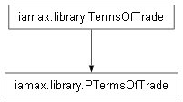

Partialized version of TermsOfTrade

Parameters: sigma (float) – Elasticity to terms-of-trade of good exports.

compute_calibrand_0(self, *, arent_final: np.ndarray, are_only_final: np.ndarray, specific_producer_prices: np.ndarray, consumer_prices: np.ndarray, consumed_volumes: np.ndarray)¶

Support the calibration of the constant scale factor implied in the terms-of-trade equation, denoted as

(213)¶\[A_X = q_{X(t=0)} \left( \frac{p_{X(t=0)}}{p_{M(t=0)}} \right)^\sigma\]

where \(q_{X(t=0)}\) is the consumed volume of exported quantity, \(p_{X(t=0)}/p_{M(t=0)}\) the price ratio of the latter against its imported counterpart and \(\sigma\) the elasticity to terms-of-trade of good exports, set at instantiation.

Parameters

arent_final (numpy.ndarray) – \((\btxta_k)_{k \in \mcI_j}\), i.e. the \(j\)th \(1 \times |\mcI_j|\) arent_final’s slice.
are_only_final (numpy.ndarray) – \((\textbf{f}_k)_{k \in \mcI_j}\), i.e. a \(j\)-th \(1 \times |\mcI_j|\) are_only_final’s slice.
specific_producer_prices (numpy.ndarray) – \((\tbP^{T}_{k,j})_{k \in \mcI_j}\), i.e. a \(j\)-th \(1 \times |\mcI_j|\) specific_producer_prices’s slice.
consumer_prices (numpy.ndarray) – \((\tbP_{k,j})_{k \in \mcI_j}\), i.e. a \(j\)-th \(1 \times |\mcI_j|\) consumer_prices’s slice.
consumed_volumes (numpy.ndarray) – \((\bQ^{T}_{k,j})_{k \in \mcI_j}\), i.e. a \(j\)th \(1 \times |\mcI_j|\) slice of consumed_volumes.

output_volume_rooter(self, specific_producer_prices: np.ndarray, consumer_prices: np.ndarray, consumed_volumes: np.ndarray, consumed_volumes_drates: np.ndarray)¶

Terms-of-trade based constraint regarding exported quantities, as follows

(214)¶\[q_{X(t)} = A_X \left( \frac{p_{M(t)}}{p_{X(t)}} \right)^\sigma \left(1 + \epsilon_{X(t)}\right)\]

Parameters

specific_producer_prices (numpy.ndarray) – \((\tbP^{T}_{k,j})_{k \in \mcI_j}\), i.e. a \(j\)-th \(1 \times |\mcI_j|\) specific_producer_prices’s slice.
consumer_prices (numpy.ndarray) – \((\tbP_{k,j})_{k \in \mcI_j}\), i.e. a \(j\)-th \(1 \times |\mcI_j|\) consumer_prices’s slice.
consumed_volumes (numpy.ndarray) – \((\bQ^{T}_{k,j})_{k \in \mcI_j}\), i.e. a \(j\)th \(1 \times |\mcI_j|\) slice of consumed_volumes.
consumed_volumes_drates (numpy.ndarray) – \((\bQ^{T, \text{drate}}_{k,j})_{k \in \mcI_j}\), i.e. a \(j\)th \(1 \times |\mcI_j|\) slice of consumed_volumes_drates, one component of which echoes \(\epsilon_X\) above.

class iamax.library.DynamicStock(delta: float, grpot: float = 0.0, dyear0: float = 1.0)¶

Example case mobilized dynamic stock abstraction.

Parameters

delta (float) – Annual depreciation rate.
grpot (float) – Annual growth potential. To .0 by default.
dyear0 (float) – Yearly recurrence period of the flux under consideration at time t=0. To 1. by default.

capacity_computer(self, *, capacities: np.ndarray, capacities_drates: np.ndarray, ordinal_volumes: np.ndarray, t: int, dyear: float)¶

s/e., \(1 \times 1\), denoted as

(215)¶\[\hq_t = \hq_{t-1}(1 - \delta)^{(y_t - y_{t-1})} + q_{t-1} \hq^{\text{drate}}_t\]

where \(\hq\) is the stock of interest, \(y_t - y_{t-1}\) stands for dyear below, \(\hq^{\text{drate}}_t\) and \(q_{t-1}\) are a \(q\)-to-\(\hq\) factor of transformation and a contributory flow at time \(t - 1\) and \(t\) respectively.

Parameters

capacities (numpy.ndarray) – \((\hbq_k)_{k \in \mcI_j}\), i.e. the \(j\)th \(|\mcL| \times |\mcI_j|\) capacities’s slice.
capacities_drates (numpy.ndarray) – \((\hbq^{\text{drate}}_k)_{k \in \mcI_j}\), i.e. a \(j\)th \(|\mcL| \times |\mcI_j|\) slice of capacities_drates (i.e. available_volumes_drates).
ordinal_volumes (numpy.ndarray) – \((\bq_k)_{k \in \mcI_j}\), i.e. the \(j\)th \(|\mcL| \times |\mcI_j|\) slice of ordinal_volumes.
t (int) – Year-targeting integer index. Cf. t, i.e. a _ilocalizations’s integer element.
dyear (float) – Number of years between t and max(0, t - 1). Cf. dyear.

Important

Since t is invoked, non-scalar arguments all consist of (column-bound) time series, the first and the second of which respectively refer to that of \(\hq\) and \(q\), as explained here.

Note

This method is vectorization friendly over the -3th axis, if any.

Example

Let’s first define the arrays awaited by the current method. The capacities

>>> caps = np.array([
...     [[0.,           0.]],
...     [[1233321.6224, 0.]],
...     [[0.,           0.]],
... ])

Idem regarding their companion driving rates (above arbitrarily interpreted as related to the notion of transformation/conversion), i.e. capacities_drates

>>> caps_drates = np.array([
...     [[0.,     0.]],
...     [[0.,     0.]],
...     [[3.7436, 0.]],
... ])

Finally, the contributory flow, assumed to derive from ordinal_volumes,

>>> ovols = np.array([
...     [[0., 0.]],
...     [[0., 87922.7702]],
...     [[0., 0.]],
... ])

Let’s finally get a DynamicStock instance and vertue the ongoing example by computing the capacity at time t.

>>> ds              = DynamicStock(delta=.04)
>>> caps[2, ..., 0] = ds.capacity_computer(
...     capacities=caps, capacities_drates=caps_drates,
...     ordinal_volumes=ovols, t=2, dyear=5.
... )
>>> caps
array([[[      0.  ,       0.  ]],
       [[1233321.62,       0.  ]],
       [[1422687.23,       0.  ]]])

Let’s vectorize the above example, keeping in mind that the temporal axis must remain first (hence the numpy.ndarray.swapaxes below).

>>> caps[2, ..., 0] = 0
>>> (vcaps := np.stack([caps, .1*caps]).swapaxes(1, 0))
array([[[[      0.  ,       0.  ]],
        [[      0.  ,       0.  ]]],
       [[[1233321.62,       0.  ]],
        [[ 123332.16,       0.  ]]],
       [[[      0.  ,       0.  ]],
        [[      0.  ,       0.  ]]]])
>>> (vovols := np.stack([ovols, .1*ovols]).swapaxes(1, 0))
array([[[[    0.  ,     0.  ]],
        [[    0.  ,     0.  ]]],
       [[[    0.  , 87922.77]],
        [[    0.  ,  8792.28]]],
       [[[    0.  ,     0.  ]],
        [[    0.  ,     0.  ]]]])
>>> (vcaps_drates := np.stack(2*[caps_drates]).swapaxes(1, 0))
array([[[[0.  , 0.  ]],
        [[0.  , 0.  ]]],
       [[[0.  , 0.  ]],
        [[0.  , 0.  ]]],
       [[[3.74, 0.  ]],
        [[3.74, 0.  ]]]])
>>> vds   = DynamicStock(delta=np.array([[[.04]], [[.08]]]))
>>> ncaps = vds.capacity_computer(
...     capacities=vcaps, capacities_drates=vcaps_drates,
...     ordinal_volumes=vovols, t=2, dyear=5.
... )
>>> ncaps
array([[[1422687.23]],
       [[ 122992.99]]])
>>> vcaps[(2, ((0,), (1,)), ..., 0)] = ncaps
>>> vcaps.shape
(3, 2, 1, 2)
>>> vcaps[(2, ((0,), (1,)), ..., 0)].shape
(2, 1, 1)
>>> vcaps
array([[[[      0.  ,       0.  ]],
        [[      0.  ,       0.  ]]],
       [[[1233321.62,       0.  ]],
        [[ 123332.16,       0.  ]]],
       [[[1422687.23,       0.  ]],
        [[ 122992.99,       0.  ]]]])

class iamax.library.OPricedDynamicStock¶

Inheritance diagram of iamax.library.OPricedDynamicStock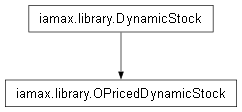

Augmented version of DynamicStock whose contributory flows’ (ordinal) prices determine its price.

static output_price_computer(ordinal_prices_transpose_lagged: float)¶: Identity method.

class iamax.library.L1NzIntDrivenDemands¶

Inheritance diagram of iamax.library.L1NzIntDrivenDemands

Class that abstracts the idea of Hicksian-like demands whose price and level characteristics are derived from their L1 normalized ioq_intensities with respect to a good located an arbitrary number of permutations away in the consumption space.

static input_volumes_computer(output_volume: np.ndarray, ioq_intensities: np.ndarray)¶

s/e.

Parameters

output_volume (float) – \(q_j\), i.e. the \(j\)th \(1 \times 1\) output_volumes’s element.
ioq_intensities (numpy.ndarray) – \((\balpha_{k,j})_{k \in \mcI_j}\), i.e. the \(j\)th \(1 \times |\mcI_j|\) ioq_intensities’s slice.

class iamax.library.O2STxRateDrivenSTxRate¶

Inheritance diagram of iamax.library.O2STxRateDrivenSTxRate

Sales tax rate whose value is determined by that of a good being two permutations away in the consumption space.

(216)¶\[\frac{\ttau^{o_0}_t}{1 + \ttau^{o_0}_t} = \frac{\ttau^{o_0}_0}{1 + \ttau^{o_0}_0} - \zeta^{o_2}_t \left( \frac{\ttau^{o_2}_t}{1 + \ttau^{o_2}_t} - \frac{\ttau^{o_2}_0}{1 + \ttau^{o_2}_0} \right)\]

where \(\ttau^{o_0}\) is the so-driven sales tax markup rate, \(\ttau^{o_2}\) is the two-permutation-away good’s rate of interest and \(\zeta^{o_2}\) the relevant order \(2\) input/output value intensity.

compute_calibrand_0(self, *, sales_taxes_totals_rates: float, t: int = 0)¶

Compute (and save) the \(t=0\)’s margin (and markup) rates.

Parameters

sales_taxes_totals_rates (numpy.ndarray) – \((\hbtau_{\Sigma, k})_{k \in \{j\}\cup\mcI_j}\), i.e. a \(j\)-th \(|\mcL| \times |\{j\}\cup\mcI_j|\) slice of sales_taxes_totals_rates.
t (int) – Year-targeting integer index. Cf. t, i.e. a _ilocalizations’s integer element.

Important

This method relies on the structure of its argument.

Note

Argument t is mobilized as a trick to request the sales tax rate of the entity under edition.

Example

>>> so = O2STxRateDrivenSTxRate()
>>> so.compute_calibrand_0(
...     sales_taxes_totals_rates=np.array([[
...         0.023105133651252,  # self related
...         0.150641610514566,  # order-2 away rate
...     ]])
... )
>>> so.o0_markup_sales_tax_total_rate_0
0.023105133651252
>>> so.o0_margin_sales_tax_total_rate_0
0.02258334250439593
>>> so.o2_markup_sales_tax_total_rate_0
0.150641610514566
>>> so.o2_margin_sales_tax_total_rate_0
0.13091966181129083

sales_tax_total_rate_computer(self, *, sales_tax_total_rate: float, iov_intensity_order2: float)¶

s/e.

Parameters

sales_tax_total_rate (float) – Cf. sales_taxes_totals_rates (as markup rate).
iov_intensity_order2 (float) – Cf. iov_intensities_order2.

Example

>>> so = O2STxRateDrivenSTxRate()
>>> so.compute_calibrand_0(
...     sales_taxes_totals_rates=np.array([[
...         0.023105133651252,  # self related
...         0.150641610514566,  # order-2 away rate
...     ]])
... )
>>> so.sales_tax_total_rate_computer(
...     sales_tax_total_rate=0.540874848689871,
...     iov_intensity_order2=0.0426989104641244,
... ).item()
0.01336155939770362

class iamax.library.O2STxRateDrivenCTxRate¶

Inheritance diagram of iamax.library.O2STxRateDrivenCTxRate

Contributive tax rate whose value is determined by the sales taxe rate of a good being two permutations away in the consumption space.

(217)¶\[\otau^{o_0}_t = \otau^{o_0}_0 - \zeta^{o_2}_t \left( \frac{\ttau^{o_2}_t}{1 + \ttau^{o_2}_t} - \frac{\ttau^{o_2}_0}{1 + \ttau^{o_2}_0} \right)\]

where \(\otau^{o_0}\) is the so-driven contributive tax margin rate, \(\ttau^{o_2}\) is the two-permutation-away good’s sales tax rate of interest and \(\zeta^{o_2}\) the relevant order \(2\) input/output value intensity.

compute_calibrand_0(self, *, contrib_tax_rate: float, sales_tax_total_rate: float)¶

Compute (and save) the \(t=0\)’s margin (and markup) rates.

Parameters

contrib_tax_rate (float) – A \(j\)-targeted contrib_taxes_rates’s scalar.
sales_tax_total_rate (float) – \((\hbtau_{\Sigma, k})_{k \in \mcI_j}\), i.e. a \(j\)-th \(1 \times |\mcI_j|\) slice of sales_taxes_totals_rates.

Note

\(\mcI_j\) is assumed to be a singleton.

Example

>>> so = O2STxRateDrivenCTxRate()
>>> so.compute_calibrand_0(
...     contrib_tax_rate=0.0225833425043962,
...     sales_tax_total_rate=0.150641610514566,
... )
>>> so.o0_margin_contrib_tax_rate_0
0.0225833425043962
>>> so.o2_markup_sales_tax_total_rate_0
0.150641610514566
>>> so.o2_margin_sales_tax_total_rate_0.item()
0.13091966181129083

contrib_tax_rate_computer(self, *, sales_tax_total_rate: float, iov_intensity_order2: float)¶

s/e.

Parameters

sales_tax_total_rate (float) – Cf. sales_taxes_totals_rates (as markup rate).
iov_intensity_order2 (float) – Cf. iov_intensities_order2.

Example

>>> so = O2STxRateDrivenCTxRate()
>>> so.compute_calibrand_0(
...     contrib_tax_rate=0.0225833425043962,
...     sales_tax_total_rate=0.150641610514566,
... )
>>> so.contrib_tax_rate_computer(
...     sales_tax_total_rate=0.540874848689871,
...     iov_intensity_order2=0.0426989104641244,
... ).item()
0.013185382131176756

class iamax.library.OLabor¶: Example case-denominated composite sector’s labor.

class iamax.library.OKLProducer¶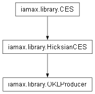: Example case-denominated domestic (intermediary) composite-&-KL good producer.

class iamax.library.OKLEProducer¶: Example case-denominated domestic (intermediary) composite-&-KLE good producer.

class iamax.library.ODProducer¶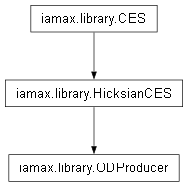: Example case-denominated domestic composite good producer.

class iamax.library.OAProducer¶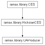: Example case-denominated armington composite good producer.

class iamax.library.ELabor¶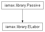: Example case-denominated energy sector’s labor.

class iamax.library.EKLProducer¶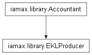: Example case-denominated domestic (intermediary) energy-&-KL good producer.

class iamax.library.EKLEProducer¶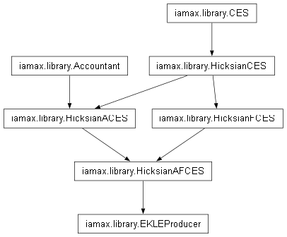: Example case-denominated domestic (intermediary) energy-&-KLE good producer.

class iamax.library.EDProducer¶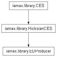: Example case-denominated domestic energy producer.

class iamax.library.EAProducer¶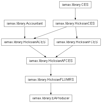: Example case-denominated armington energy producer.

class iamax.library.Consumer¶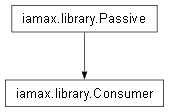: Example case-denominated final consumers.

class iamax.library.Ordinaler¶

Class that abstracts the idea of an underlying capital stock being calculated based on an assumed rental price, and an investment volume being adjusted accordingly.

static ordinal_volume_computer(input_volumes: np.ndarray)¶

Perceived index, \(1 \times 1\).

Parameters: input_volumes (numpy.ndarray) – \((\bQ_{k,j})_{k \in \mcI_j}\), i.e. the \(j\)th \(1 \times |\mcI_j|\) input_volumes’s slice.

See also

ordinal_volumes.

class iamax.library.AdditiveOrdinaler¶

s/e.

static ordinal_volume_computer(input_volumes: np.ndarray)¶

Perceived index, \(1 \times 1\), denoted as

(218)¶\[\mfq_j = \sum_{k \in \mcI_j} q_k\]

Parameters: input_volumes (numpy.ndarray) – \((\bQ_{k,j})_{k \in \mcI_j}\), i.e. the \(j\)th \(1 \times |\mcI_j|\) input_volumes’s slice.

See also

ordinal_volumes.

class iamax.library.Government¶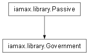: Example case-denominated public administration.

class iamax.library.Investor¶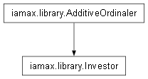: Example case-denominated investors.

class iamax.library.ImplicitLeontief¶

s/e.

compute_calibrand_0(self, *, input_volumes: np.ndarray)¶

s/e.

Parameters: input_volumes (numpy.ndarray) – \((\bQ_{k,j})_{k \in \mcI_j}\), i.e. the \(j\)th \(1 \times |\mcI_j|\) input_volumes’s slice.

compute_calibrand_0_star(self, *, additive_input_volumes_shares_drates: np.ndarray)¶

s/e.

Parameters: additive_input_volumes_shares_drates (numpy.ndarray) – \((\bQ^\text{drate}_{\%,k,j})_{k \in \mcI_j}\), i.e. the \(j\)th \(1 \times |\mcI_j|\) slice of additive_input_volumes_shares_drates.

input_volumes_computer(self, *, ordinal_volume: float|np.ndarray)¶

s/e.

Parameters: ordinal_volume (float) – \(\mfq_j\), i.e. the \(j\)th \(1 \times 1\) ordinal_volumes’s element.

class iamax.library.OImplicitLeontief¶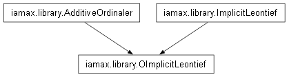: s/e.

class iamax.library.MarshallianILeo¶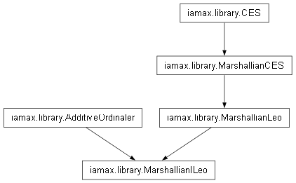: s/e.

class iamax.library.LaspeyresianGFL(negated_mask: bool = False)¶

Class that abstracts the idea of economic agents who anchor their consumption decisions to the initial period’s expenditure shares, mirroring the “fixed-weight” logic of the Laspeyres framework. This class moreover allows one to restrict (in a generalized manner) the set of trade-offs being forced.

Parameters: negated_mask (bool) – Whether the mask passed as argument input_volumes_drates2 of the method compute_calibrand_0 is to be negated. Argument input_volumes_drates2 indeed boolean-specifies the goods being freely subject to trade-off by default. Set to False by default.

compute_calibrand_0(self, *, budget_constraint: float, input_values: np.ndarray, input_volumes_drates2: np.ndarray)¶

s/e.

Parameters

budget_constraint (float) – \(r_j\), i.e. the \(j\)th \(1 \times 1\) budget_constraints’s element.
input_values (numpy.ndarray) – \((\bmcV_{k,j})_{k \in \mcI_j}\), i.e. the \(j\)th \(1 \times |\mcI_j|\) input_values’s slice.
input_volumes_drates2 (numpy.ndarray) – \((\bQ^\text{drate}_{k,j})_{k \in \mcI_j}\), i.e. the \(j\)th \(1 \times |\mcI_j|\) input_volumes_drates2’s slice. This variable is coerced into boolean and used as mask.

Example

>>> budc  = 200.
>>> ivals = np.array([[110., 80., 10.]])
>>> imsks = np.array([[1, 1, 1]])

>>> c = LaspeyresianGFL(negated_mask=False).compute_calibrand_0(
...     budget_constraint=budc, input_values=ivals,
...     input_volumes_drates2=imsks
... )
>>> c.calibrand_0
array([[0.55, 0.4 , 0.05]])

Let’s then illustrate how such calculation can be vectorized.

>>> vbudc  = np.array([[[budc]], [[budc]]])
>>> vivals = np.stack((ivals, ivals))
>>> vimsks = np.stack((imsks, np.array([[1, 0, 1]])))
>>> c.compute_calibrand_0(
...     budget_constraint=vbudc, input_values=vivals,
...     input_volumes_drates2=vimsks
... ).calibrand_0
array([[[0.55, 0.4 , 0.05]],
       [[0.92, 0.  , 0.08]]])

input_values_shares_rooter(self, *, budget_constraint: float, input_values: np.ndarray)¶

Input demands, \(1 \times |\mcI_j|\)

Parameters

budget_constraint (float) – \(r_j\), i.e. the \(j\)th \(1 \times 1\) budget_constraints’s element.
input_values (numpy.ndarray) – \((\bmcV_{k,j})_{k \in \mcI_j}\), i.e. the \(j\)th \(1 \times |\mcI_j|\) input_values’s slice.

Example

>>> ivals = np.array([[110., 60., 20., 10.]])
>>> budc  = ivals.sum()
>>> c1111 = LaspeyresianGFL(
...     negated_mask=False
... ).compute_calibrand_0(
...     budget_constraint=budc, input_values=ivals,
...     input_volumes_drates2=np.array([[1, 1, 1, 1]])
... )
>>> c1111.calibrand_0
array([[0.55, 0.3 , 0.1 , 0.05]])
>>> c1001 = LaspeyresianGFL(
...     negated_mask=False
... ).compute_calibrand_0(
...     budget_constraint=budc, input_values=ivals,
...     input_volumes_drates2=np.array([[1, 0, 0, 1]])
... )
>>> c1001.calibrand_0
array([[0.92, 0.  , 0.  , 0.08]])

>>> ivals *= np.array([[1, 5/6, 3/2, 1]])
>>> budc   = ivals.sum()
>>> c1111.input_values_shares_rooter(
...     budget_constraint=budc, input_values=ivals,
... )
array([[ 0.  , -0.13,  0.27,  0.  ]])
>>> c1001.input_values_shares_rooter(
...     budget_constraint=budc, input_values=ivals,
... )
array([[0., 0., 0., 0.]])

class iamax.library.EExporter¶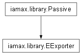: Example case-denominated exporters of energy goods.

class iamax.library.OExporter¶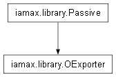: Example case-denominated exporters of composite goods.

class iamax.library.OneToOne(intensity_factor: float = 1.0)¶

Abstraction that grants the properties (defined by the methods below) of one entity to another.

Parameters: intensity_factor (float) – S/e. set to 1 by default.

input_volume_computer(self, *, output_volume: float)¶

Identity function (to within a multiplicative intensity_factor).

Parameters

output_volume (float) – \(q_j\), i.e. the \(j\)th \(1 \times 1\) output_volumes’s element.

Example

>>> OneToOne().input_volume_computer(output_volume=.5)
0.5
>>> OneToOne(2).input_volume_computer(output_volume=.5)
1.0

class iamax.library.AOneToOne¶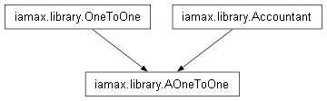: Augmented version of OneToOne that deals with prices following Accountant’s approach.

class iamax.library.OnBoard¶

Inheritance diagram of iamax.library.OnBoard

Free-on-board (FOB) to Cost-Insurance-and-Freight (CIF).

compute_calibrand_0(self, *, producer_net_price_drate: np.ndarray, purchaser_prices: np.ndarray)¶

s/e.

Important

This method relies on the structure of its argument, with the transported good volume being the first arrays’ component.

Example

>>> oprc  = 0.038
>>> pprcs = np.array([[0.774, 0.68]])
>>> ob    = OnBoard()
>>> ob.compute_calibrand_0(
...     producer_net_price_drate=oprc,
...     purchaser_prices=pprcs
... )
>>> ob.calibrand_0
array([[0.04]])

Let’s vectorize the above example.

>>> voprc  = np.array([[[oprc]], [[2*oprc]]])
>>> vpprcs = np.stack((pprcs, 2*pprcs))
>>> ob.compute_calibrand_0(
...     producer_net_price_drate=voprc,
...     purchaser_prices=vpprcs
... )
>>> ob.calibrand_0
array([[[0.04]],
       [[0.09]]])

input_volumes_computer(self, *, output_volume: float)¶

s/e.

Important

This method relies on the structure of its argument, with the transported good volume being the first arrays’ component.

Example

>>> oprc  = 0.038
>>> pprcs = np.array([[0.774, 0.68]])
>>> ob    = OnBoard()
>>> ob.compute_calibrand_0(
...     producer_net_price_drate=oprc,
...     purchaser_prices=pprcs
... )

>>> ovol  = 197432.592
>>> ivols = ob.input_volumes_computer(
...     output_volume=ovol
... )
>>> ivols
array([[197432.59,   8539.54]])
>>> ivols.shape
(1, 2)

Let’s vectorize the above example.

>>> voprc  = np.array([[[oprc]], [[2*oprc]]])
>>> vpprcs = np.stack((pprcs, 2*pprcs))
>>> ob.compute_calibrand_0(
...     producer_net_price_drate=voprc,
...     purchaser_prices=vpprcs
... )
>>> vovol  = np.array([[[ovol]], [[2*ovol]]])
>>> vivols = ob.input_volumes_computer(
...     output_volume=vovol
... )
>>> vivols
array([[[197432.59,   8539.54]],
       [[394865.18,  34158.16]]])
>>> vivols.shape
(2, 1, 2)

class iamax.library.IOnBoard¶

Inheritance diagram of iamax.library.IOnBoard

Transport-intensity calibrated version of OnBoard

compute_calibrand_0(self, *, input_volumes: np.ndarray)¶

s/e.

Important

This method relies on the structure of its argument, with the transported good volume being the first arrays’ component.

Example

>>> ivols = np.array([[3., 6.]])
>>> ob    = IOnBoard()
>>> ob.compute_calibrand_0(
...     input_volumes=ivols
... )
>>> ob.calibrand_0
array([[2.]])

Let’s vectorize the above example.

>>> vivols = np.stack((ivols, [[3., .0]]))
>>> ob.compute_calibrand_0(
...     input_volumes=vivols
... )
>>> ob.calibrand_0
array([[[2.]],
       [[0.]]])

class iamax.library.CorrTrader¶

Trader abstraction whose optimal demands derive from a portfolio correlated allocation problem.

compute_qois(self, *, budget_constraints: np.ndarray, input_prices: np.ndarray, ioq_intensities_drates: np.ndarray, ordinal_volumes_drates: np.ndarray)¶

s/e.

Example

>>> bcons = np.ones((1, 3)) / 3
>>> iprcs = np.identity(3)
>>> beta  = np.ones((3, 3)) / 6
>>> ovdrs = np.zeros((1, 3))
>>> ct = CorrTrader()
>>> ct.compute_qois(
...     budget_constraints=bcons,
...     input_prices=iprcs,
...     ioq_intensities_drates=beta,
...     ordinal_volumes_drates=ovdrs,
... ).input_volumes_computer()
array([[0.33, 0.  , 0.  ],
       [0.  , 0.33, 0.  ],
       [0.  , 0.  , 0.33]])
>>> ct.ordinal_volumes_computer()
array([[0.67, 0.67, 0.67]])
>>> ct.ordinal_prices_computer()
array([[0.5, 0.5, 0.5]])

Let’s vectorize the above example.

>>> vbcons = np.stack((bcons, 2*bcons))
>>> viprcs = np.stack((iprcs, .5*iprcs))
>>> betas  = np.stack((beta, beta / 2))
>>> vovdrs = np.stack((ovdrs, ovdrs))
>>> ct.compute_qois(
...     budget_constraints=vbcons,
...     input_prices=viprcs,
...     ioq_intensities_drates=betas,
...     ordinal_volumes_drates=vovdrs,
... ).input_volumes_computer()
array([[[0.33, 0.  , 0.  ],
        [0.  , 0.33, 0.  ],
        [0.  , 0.  , 0.33]],
       [[1.33, 0.  , 0.  ],
        [0.  , 1.33, 0.  ],
        [0.  , 0.  , 1.33]]])
>>> ct.ordinal_volumes_computer()
array([[[0.67, 0.67, 0.67]],
       [[5.33, 5.33, 5.33]]])
>>> ct.ordinal_prices_computer()
array([[[0.5 , 0.5 , 0.5 ]],
       [[0.12, 0.12, 0.12]]])

input_volumes_computer(self)¶: s/e.

ordinal_volumes_computer(self)¶: s/e.

ordinal_prices_computer(self)¶: s/e.

library¶

`library`¶